Abaqus Plug-In (`desicos.abaqus`)¶

The desicos.abaqus module includes the DESICOS plug-in for Abaqus whose functionalities can be used in two main ways, using the Graphic User Interface (GUI) or using the Python API.

ConeCyl (`desicos.abaqus.conecyl`)¶

Cone/Cylinder Model¶

Figure 1 provides a schematic view of the typical model created using this module. Two coordinate systems are defined: one rectangular with axes $X_1$ , $X_2$ , $X_3$ and a cylindrical with axes $R$ , $Th$ , $Z$ .

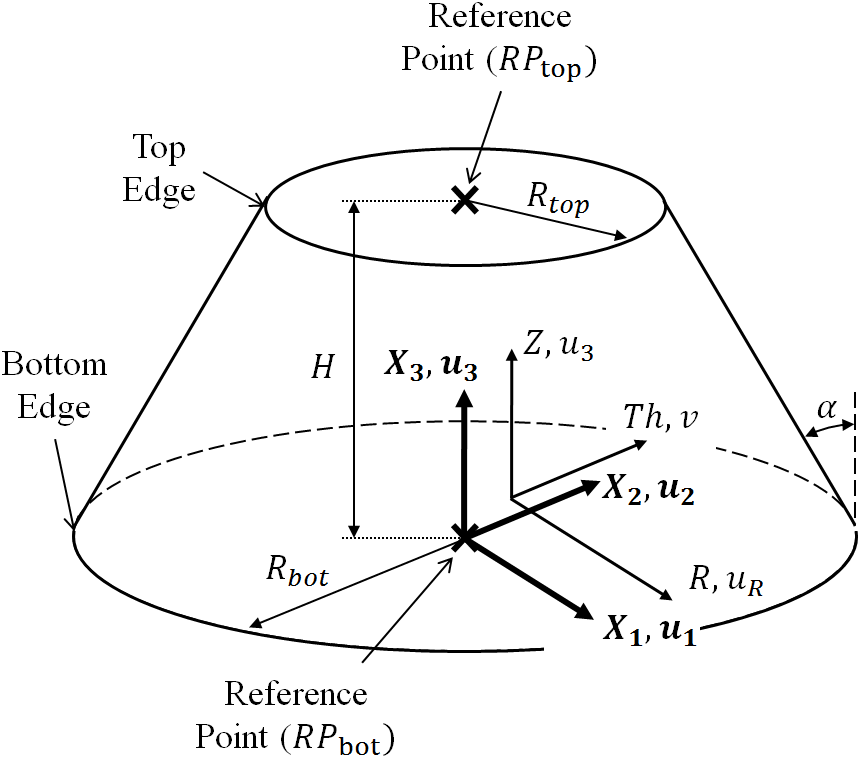
Figure 1: Cone/Cylinder Model¶

The complexity of the actual model created in Abaqus goes beyond the simplification above

Boundary Conditions¶

Based on the coordinate systems shown in Figure 1 the following boundary condition parameters can be controlled:

constraint for radial and circumferential displacement ( $u_R$ and $v$ ) at the bottom and top edges
simply supported or clamped bottom and top edges, consisting in the rotational constraint along the meridional coordinate, called $\phi_x$ .
use of resin rings as described in the next section
the use of distributed or concentrated load at the top edge will be automatically determined depending on the attributes of the current ConeCyl object

application of shims at the top edge as detailed in ImpConf.add_shim_top_edge(), following this example:

from desicos.abaqus.conecyl import ConeCyl

cc = ConeCyl()
cc.from_DB('castro_2014_c02')
cc.impconf.add_shim(thetadeg, thick, width)

application of uneven top edges as detailed in UnevenTopEdge.add_measured_u3s(), following this example:

thetadegs = [0.0, 22.5, 45.0, 67.5, 90.0, 112.5, 135.0, 157.5, 180.0,
             202.5, 225.0, 247.5, 270.0, 292.5, 315.0, 337.5, 360.0]
u3s = [0.0762, 0.0508, 0.1270, 0.0000, 0.0000, 0.0762, 0.2794, 0.1778,
       0.0000, 0.0000, 0.0762, 0.0000, 0.1016, 0.2032, 0.0381, 0.0000,
       0.0762]
cc.impconf.add_measured_u3s_top_edge(thetadegs, u3s)

Resin Rings¶

When resin rings are used the actual boundary condition will be determined by the parameters defining the resin rings (cf. Figure 2), and therefore no clamped conditions will be applied in the shell edges.

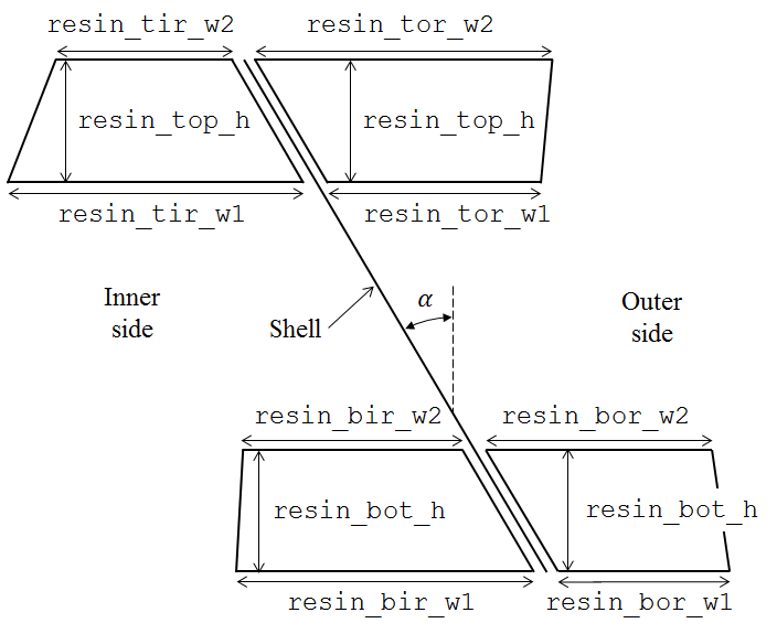
Figure 2: Resin Rings¶

Defining resin rings can be done following the example below, where each attribute is detailed in the ConeCyl class description:

from desicos.abaqus.conecyl import ConeCyl

cc = Conecyl()
cc.from_DB('castro_2014_c02')
cc.resin_add_BIR = False
cc.resin_add_BOR = True
cc.resin_add_TIR = False
cc.resin_add_TOR = True
cc.resin_E = 2454.5336
cc.resin_nu = 0.3
cc.resin_numel = 3
cc.resin_bot_h = 25.4
cc.resin_top_h = 25.4
cc.resin_bir_w1 = 25.4
cc.resin_bir_w2 = 25.4
cc.resin_bor_w1 = 25.4
cc.resin_bor_w2 = 25.4
cc.resin_tir_w1 = 25.4
cc.resin_tir_w2 = 25.4
cc.resin_tor_w1 = 25.4
cc.resin_tor_w2 = 25.4

The ConeCyl Class¶

class desicos.abaqus.conecyl.conecyl.ConeCyl[source]¶

ConeCyl object

Carries all the information necessary to create a finite element model for the analysis of conical and cylindrical structures. The tables below show the attributes grouped by category.

General Attributes	Description
`name_DB`	`str`, name of the corresponding `desicos.conecylDB.ccs` entry
`model_name`	`str`, Name of the corresponding model in Abaqus
`rename`	`bool`, tells to automatically rename during `rebuild()`
`rebuilt`	`bool`, tells if `rebuild()` already finished
`created_model`	`bool`, tells if the corresponding model was already created in Abaqus
`impconf`	The corresponding imperfection configuration (see `ImpConf`)
`stringerconf`	The corresponding stringer configuration (see `StringerConf`)

Geometric Attributes	Description
`rbot`	Radius at the bottom edge
`rtop`	Radius at the top edge
`H`	Height
`L`	Meridional length (same as `H` for cylinders)
`alphadeg`	Cone semi-vertex angle in degrees

Laminate Attributes	Description
`stack`	`list`, stacking sequence with angles in degrees
`plyt`	`float`, ply thickness that will be used for all plies
`plyts`	`list`, ply thicknesses for each ply (overwrites `plyt` if both are given). If this has a different length than `stack`, the first thickness will be applied for all plies
`laminapropKey`	`str`, name of the lamina properties contained in the database (see `conecylDB.laminaprops`
`laminapropKeys`	`list` a list of strings when different lamina property names are given for each ply (overwrites `laminapropKey` when given)
`laminaprop`	`tuple`, lamina properties given as `(E11, E22, nu12, G12, G13, G23)`
`laminaprops`	`list` a list of tuples when different lamina properties should be used for each ply (overwrites `laminaprop`, `laminapropKey` and `laminapropKeys`, when given)
`allowable`	`tuple`, lamina allowables given as `(S11t, S11c, S22t, S22c, S12, S13)`
`allowables`	`list` a list of tuples when different lamina allowables should be used for each ply

Load	Description
`displ_controlled`	`bool`, if the axial compression is displacement controlled
`pressure_load`	`float`, the pressure load to be applied (a positive value will create a positive pressure, if `None, False, 0` no pressure is applied)
`pressure_step`	`int`, if pressure should be applied in the first (constant) or second (incremented) step
`axial_displ`	`float`, the axial displacement Note Applicable if `displ_controlled=True`
`axial_load`	`float`, the axial load Note Applicable if `displ_controlled=False`
`axial_step`	`int`, if the axial load should be applied in the first (constant) or second (incremented) step
`Nxxtop`	`str`, allows the use of a general equation for the distributed force $N_{xx}$ at the top edge. The coordinates of the top edge are given in cylindrical coordinates: `R`, `Th`, `Z`; and common functions like `cos`, `sin`, `tan`, `acos`, `asin`, `atan`, `pow` and constants like `pi`, `e` etc can be used. Example: cc.Nxxtop = "cos(Th)+sin(Th)" Note If `Nxxtop` is not given, the formula: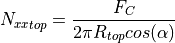 ${N_{xx}}_{top} = \frac{F_C}{2 \pi R_{top} cos(\alpha)}$ will be adopted, where $F_C$ is the `axial_load` attribute Note Applicable if `displ_controlled=False`
`Nxxtop_vec`	`tuple`, the direction to apply `Nxxtop`. Applicable only when `Nxxtop` is defined. This vector is defined with two points in the cylindrical coordinate system of Figure 1: $((R_1, Th_1, Z_1), (R_2, Th_2, Z_2))$ If no direction is given `Nxxtop` will be applied along the shell membrane direction Note Applicable if `displ_controlled=False`
`linear_buckling`	`bool`, tells if the current model is for linear buckling analysis. If `True` the created model will have no imperfection and only an unitary axial load applied at the top edge

Note

The routines automatically determine whether the load should be distributed or applied in a reference point based on the defined boundary conditions

Boundary Conditions	Description
`bc_fix_bottom_uR`	`bool`, if the radial displacement should be constrained at the bottom edge (cf. Figure 1)
`bc_fix_bottom_v`	`bool`, if the circumferential displacement should be constrained at the bottom edge (cf. Figure 1)
`bc_bottom_clamped`	`bool`, if the bottom edge should be clamped Note Until version 2.1.3 (inclusive), this setting would not apply if `cc.resin_add_BIR or cc.resin_add_BOR`
`bc_fix_bottom_side_uR`	`bool`, if the radial displacement should be constrained at the inner / outer side faces of the bottom resin rings (when present).
`bc_fix_bottom_side_v`	`bool`, if the circumferential displacement should be constrained at the inner / outer side faces of the bottom resin rings (when present).
`bc_fix_bottom_side_u3`	`bool`, if the vertical displacement should be should be constrained at the inner / outer side faces of the bottom resin rings (when present).
`bc_fix_top_uR`	`bool`, if the radial displacement should be constrained at the top edge (cf. Figure 1)
`bc_fix_top_v`	`bool`, if the circumferential displacement should be constrained at the top edge (cf. Figure 1)
`bc_top_clamped`	`bool`, if the top edge should be clamped Note Until version 2.1.3 (inclusive), this setting would not apply if `cc.resin_add_TIR or cc.resin_add_TOR`
`bc_fix_top_side_uR`	`bool`, if the radial displacement should be constrained at the inner / outer side faces of the top resin rings (when present).
`bc_fix_top_side_v`	`bool`, if the circumferential displacement should be constrained at the inner / outer side faces of the top resin rings (when present).
`bc_fix_top_side_u3`	`bool`, if the vertical displacement should be should be constrained at the inner / outer side faces of the top resin rings (when present).

Resin Rings	Description (the attributes are illustrated here)
`resin_add_BIR`	`bool`, tells if a resin ring should be added to the inner part of the bottom edge
`resin_add_BOR`	`bool`, tells if a resin ring should be added to the outer part of the bottom edge
`resin_add_TIR`	`bool`, tells if a resin ring should be added to the inner part of the top edge
`resin_add_TOR`	`bool`, tells if a resin ring should be added to the outer part of the top edge
`resin_numel`	Number of solid elements in the resin ring
`resin_E`	Young modulus of the resin material
`resin_nu`	Poisson ratio of the resin material
`resin_bot_h`	Thickness of the bottom resin ring
`resin_top_h`	Thickness of the top resin ring
`resin_bir_w1`	Lower face width of the bottom inner ring
`resin_bir_w2`	Upper face width of the bottom inner ring
`resin_bor_w1`	Lower face width of the bottom outer ring
`resin_bor_w2`	Upper face width of the bottom outer ring
`resin_tir_w1`	Lower face width of the top inner ring
`resin_tir_w2`	Upper face width of the top inner ring
`resin_tor_w1`	Lower face width of the top outer ring
`resin_tor_w2`	Upper face width of the top outer ring
`use_DLR_bc`	Apply boundary conditions used at DLR. It consists on using all the resin rings plus radial constraints only on the side faces of the resin.

Mesh Parameters	Description
`numel_r`	Number of elements around the circumference. This is sufficient to define the whole mesh size since the algorithms will keep an element aspect-ratio close to 1:1
`elem_type`	Element type. Tested with: `'S4'`, `'S4R'`, `'S8R'`, `'S8R5'`

The analysis will be divided in one or two steps, and the corresponding analysis parameters for each step are ending with 1 or 2. When only one step is used the parameters corresponding to step 2 will be applied.

Analysis Parameters	Description
`separate_load_steps`	`bool`, tells if the load steps should be separated into two: constant loads incremented loads
`initialInc1`	Initial increment size for step 1
`initialInc2`	Initial increment size for step 2
`minInc1`	Minimum increment size for step 1
`minInc2`	Minimum increment size for step 2
`maxInc1`	Maximum increment size for step 1
`maxInc2`	Maximum increment size for step 2
`maxNumInc1`	Maximum number of increments for step 1
`maxNumInc2`	Maximum number of increments for step 2
`damping_factor1`	If $\ne$ `None` artificial damping will be applied to step 1
`damping_factor2`	If $\ne$ `None` artificial damping will be applied to step 2
`timeInterval`	`float`, the time interval where the outputs will be printed
`stress_output`	`bool`, tells to print stress outputs
`force_output`	`bool`, tells to print force outputs
`output_requests`	`list`, contains all the output variables that will be printed in the output
`ncpus`	Number of CPUs to run the jobs

Methods

`attach_results`()	Attach the odb file into Abaqus
`calc_ABD_matrix`()	Calculates the laminate stiffness matrix (ABD matrix)
`calc_SPL_prediction`()	Calculates the predicted values for P1 and N1 based on empirically obtained formulae
`calc_nasaKDF`()	Calculates the KDF using the NASA SP-8007 guideline
`calc_partitions`([thetadegs, pts])	Updates all circumferential and axial positions to partition
`create_model`([force])	Triggers the routines to create the model in Abaqus
`detach_results`(odb)	Detach an odb file from Abaqus
`extract_fiber_orientation`(ply_index, …)	Get the fiber orientation at the centroid of each element
`extract_field_output`([ignore])	Extract the current field output for a cylinder/cone from Abaqus
`extract_msi_data`()	Get a data grid representing the nodal offsets w.r.t.
`extract_thickness_data`()	Get the thickness at the centroid of each element
`fr`(z)	Calculates the radius at a given `z` position
`from_DB`([name_DB])	Fetch all the cone/cylinder data from the database
`get_step_name`(step)	Get the step name corresponding to an integer number
`plot_current_field_opened`([ignore, plot_type])	Print the current field output for a cylinder/cone model from Abaqus
`plot_field_data`(x, y, field[, …])	Print data field output to a file
`plot_msi_opened`([plot_type])	Make an opened MSI (mid-surface imperfection) plot from the current conecyl model
`plot_orientation_opened`(ply_index, use_elements)	Make a fiber orientation plot from the current cone model
`plot_thickness_opened`([plot_type])	Make an opened thickness plot from the current conecyl model
`prepare_to_save`()	Prepare the `ConeCyl` to be saved
`r_z_from_pt`([pt])	Radius and the axial position from a given normalized position
`rebuild`([force, save_rebuild])	Updates the properties of the current `ConeCyl` object
`transform_plot_data`(thetas, zs, values, …)	Transform coordinates of plot data, to prepare for plotting
`write_job`([submit, wait, multiple_cores])	Writes the job of the corresponding Abaqus model

check_completed
plot_displacements
plot_forces
plot_stress_analysis
plot_xy
read_outputs
read_walltime
stress_analysis

attach_results()[source]¶

Attach the odb file into Abaqus

If the odb file exists it will be attached in session.odbs, in Abaqus.

Note

Must be called from Abaqus

calc_ABD_matrix()[source]¶

Calculates the laminate stiffness matrix (ABD matrix)

Requires that all the laminate attributes are defines.

Returns

lamLaminate object.

calc_SPL_prediction()[source]¶

Calculates the predicted values for P1 and N1 based on empirically obtained formulae

Here P1 is the perturbation load (in N) at which a local snap-through (LST) appears at an axial load level equal to the global buckling load. N1 is the global buckling load that is obtained with P1 applied.

Returns

outtuple: 2-tuple, containing the calculated values for P1 and N1

Notes

The empirical formulae (for now) do not take the full set of laminate properties (A, B, D) into account. Instead, the equivalent orthotropic material is calculated (based on the A-matrix only) and used in the formulae.

calc_nasaKDF()[source]¶

Calculates the KDF using the NASA SP-8007 guideline

Returns

nasaKDFfloat: The knock-down factor (KDF) calculates using the NASA SP-8007.

calc_partitions(thetadegs=None, pts=None)[source]¶

Updates all circumferential and axial positions to partition

This method reads all the imperfections and collects the circumferential positions thetadegs and the normalized meridional positions pts where partitions should be created. These two lists will be used in the routines to create an Abaqus model.

Parameters

thetadegslist or None, optional: Additional positions where circumferential partitions are desired
ptslist or None, optional: Additional positions where meridional partitions are desired

create_model(force=False)[source]¶

Triggers the routines to create the model in Abaqus

The auxiliary module _create_model.py is used, from where the functions _create_mesh(), _create_load_steps() and _create_loads_bcs() are executed in this order.

Note

Must be called from Abaqus

Note

When new functionalities have to be implemented or for any debugging purposes, one can conveniently change file _create_model.py directly, and using the __main__ section at the end of this file makes it easy to test whatever necessary methods. The tests can be repeatedly run doing:

import os

from desicos.abaqus.constants import DAHOME
os.chdir(os.path.join(DAHOME, 'conecyl'))
execfile('_create_model.py')

Parameters

forcebool, optional: Forces the model creation even if the finite element model corresponding to this ConeCyl object already exists.

detach_results(odb)[source]¶

Detach an odb file from Abaqus

Note

Must be called from Abaqus

Parameters

odbAbaqus’ Odb object.

extract_fiber_orientation(ply_index, use_elements)[source]¶

Get the fiber orientation at the centroid of each element

Parameters

ply_indexint: Index of the ply of interest
use_elementsbool: If True, use the actual element centroids (from Abaqus) If False, estimate their locations instead.

Returns

outtuple: Where out[0] and out[1] contain the circumferential (theta) and vertical (z) coordinates and out[2] the corresponding values.

Notes

Must be called from Abaqus if use_elements == True

extract_field_output(ignore=[])[source]¶

Extract the current field output for a cylinder/cone from Abaqus

Parameters

ignorelist, optional: A list with the node ids to be ignored. It must contain any nodes outside the mapped mesh included in parts['part_name_shell'].nodes.

Returns

outtuple: Where out[0] and out[1] contain the circumferential (theta) and vertical (z) coordinates and out[2] the corresponding values.

extract_msi_data()[source]¶

Get a data grid representing the nodal offsets w.r.t. the reference surface, caused by mid-surface imperfection(s).

Returns

outtuple: Where out[0] and out[1] contain the circumferential (theta) and vertical (z) coordinates and out[2] the corresponding imperfection offsets.

Notes

Must be called from Abaqus

extract_thickness_data()[source]¶

Get the thickness at the centroid of each element

Returns

outtuple: Where out[0] and out[1] contain the circumferential (theta) and vertical (z) coordinates and out[2] the corresponding thicknesses.

Notes

Must be called from Abaqus

fr(z)[source]¶

Calculates the radius at a given z position

Parameters

zfloat: Axial position from bottom to top.

Returns

rfloat: The calculated radius.

from_DB(name_DB='')[source]¶

Fetch all the cone/cylinder data from the database

Parameters

name_DBstr: Name of the corresponding desicos.conecylDB.ccs entry.

Returns

ccConeCyl object with the updated properties.

get_step_name(step)[source]¶

Get the step name corresponding to an integer number

Parameters

stepint: A step number. Abaqus’ “Initial” step does not count, such that step=1 will be the first step after the “Initial” step.

Returns

step_namestr: The step name.

plot_current_field_opened(ignore=[], plot_type=1, **kwargs)[source]¶

Print the current field output for a cylinder/cone model from Abaqus

Parameters

ignorelist, optional

A list with the node ids to be ignored. It must contain any nodes outside the mapped mesh included in parts['part_name_shell'].nodes.

plot_typeint, optional

For cylinders only 4 and 5 are valid. For cones all the following types can be used:

1: concave up (default for cones)
2: concave down
3: stretched closed
4: stretched opened ( $r(z) \times \theta$ vs. $H$ )
5: stretched opened ( $r_{bottom}$ vs. $H$ )
6: concave, starting at $\theta = 0$

kwargsdict

Other keyword args will be directly passed to plot_field_data See the documentation of that method for more details.

Returns

outtuple: Where out[0] and out[1] contain the circumferential and meridional grids of coordinates and out[2] the corresponding field output.

plot_field_data(x, y, field, create_npz_only=False, ax=None, figsize=3.3, 3.3, save_png=True, aspect='equal', clean=True, outpath='', pngname='plot_from_abaqus.png', npzname='plot_from_abaqus.npz', pyname='plot_from_abaqus.py', num_levels=400, show_colorbar=True, lines=None)[source]¶

Print data field output to a file

Parameters

xnumpy.array: Grid of x-coordinates to plot
ynumpy.array: Grid of y-coordinates to plot
fieldnumpy.array: Grid of field data to plot
create_npz_onlybool, optional: If True only the data belonging to the desired field output will be saved in a .npz file, and no plotting is performed.
axAxesSubplot, optional: When ax is given, the contour plot will be created inside it.
figsizetuple, optional: The figure size given by (width, height).
save_pngbool, optional: Flag telling whether the contour should be saved to an image file.
aspectstr, optional: String that will be passed to the AxesSubplot.set_aspect() method.
cleanbool, optional: Clean axes ticks, grids, spines etc.
outpathstr, optional: Output path where the data from Abaqus and the plots are saved (see notes).
pngnamestr, optional: The file name for the generated image file.
npznamestr, optional: The file name for the generated npz file.
pynamestr, optional: The file name for the generated Python file.
num_levelsint, optional: Number of contour levels (higher values make the contour smoother).
show_colorbarbool, optional: Include a color bar in the figure.
lineslist, optional: List of lines to draw on top of the contour plot. Each line is either a 2-tuple (list of x-coords, list of y-coords), or a 2xN numpy array.

Notes

The data is saved using np.savez() into outpath as npzname with an accompanying script for plotting pyname, very handy when Matplotlib is not importable from Abaqus.

plot_msi_opened(plot_type=1, **kwargs)[source]¶

Make an opened MSI (mid-surface imperfection) plot from the current conecyl model

Parameters

plot_typeint, optional

For cylinders only 4 and 5 are valid. For cones all the following types can be used:

1: concave up (default for cones)
2: concave down
3: stretched closed
4: stretched opened ( $r(z) \times \theta$ vs. $H$ )
5: stretched opened ( $r_{bottom}$ vs. $H$ )
6: concave, starting at $\theta = 0$

kwargsdict

Other keyword args will be passed to plot_field_data See the documentation of that method for more details.

Notes

Must be called from Abaqus

plot_orientation_opened(ply_index, use_elements, plot_type=1, **kwargs)[source]¶

Make a fiber orientation plot from the current cone model

Only valid for cones that have a ply piece imperfection.

Parameters

ply_indexint

Index of the ply of interest

use_elementsbool

If True, use the actual element centroids (from Abaqus) If False, estimate their locations instead.

plot_typeint, optional

For cones all the following types can be used:

1: concave up (default for cones)
2: concave down
3: stretched closed
4: stretched opened ( $r(z) \times \theta$ vs. $H$ )
5: stretched opened ( $r_{bottom}$ vs. $H$ )
6: concave, starting at $\theta = 0$

kwargsdict

Other keyword args will be passed to plot_field_data See the documentation of that method for more details.

Notes

Must be called from Abaqus if use_elements == True

plot_thickness_opened(plot_type=1, **kwargs)[source]¶

Make an opened thickness plot from the current conecyl model

Parameters

plot_typeint, optional

For cylinders only 4 and 5 are valid. For cones all the following types can be used:

1: concave up (default for cones)
2: concave down
3: stretched closed
4: stretched opened ( $r(z) \times \theta$ vs. $H$ )
5: stretched opened ( $r_{bottom}$ vs. $H$ )
6: concave, starting at $\theta = 0$

kwargsdict

Other keyword args will be passed to plot_field_data See the documentation of that method for more details.

Notes

Must be called from Abaqus

prepare_to_save()[source]¶

Prepare the ConeCyl to be saved

Any reference to Abaqus objects are removed in this method.

r_z_from_pt(pt=0.5)[source]¶

Radius and the axial position from a given normalized position

Parameters

ptfloat or np.ndarray: Normalized meridional position.

Returns

r, ztuple: The radius and the actual axial position at the given normalized position. It is a tuple of floats if pt is a float or a tuple of numpy.ndarray objects if pt is an array.

rebuild(force=False, save_rebuild=True)[source]¶

Updates the properties of the current ConeCyl object

Parameters

forcebool: Force the update even if it is already rebuilt (even if the rebuilt attribute is True).
save_rebuildbool: Tells if the rebuilt attribute should be True after the update.

transform_plot_data(thetas, zs, values, plot_type, wrap=True)[source]¶

Transform coordinates of plot data, to prepare for plotting

Parameters

thetasnumpy.array

Array of circumferential coordinates

zsnumpy.array

Array of vertical coordinates

valuesnumpy.array

Array of values

plot_typeint, optional

For cylinders only 4 and 5 are valid. For cones all the following types can be used:

1: concave up (default for cones)
2: concave down
3: stretched closed
4: stretched opened ( $r(z) \times \theta$ vs. $H$ )
5: stretched opened ( $r_{bottom}$ vs. $H$ )
6: concave, starting at $\theta = 0$

wrapbool, optional

If True, wrap $\theta$ -coordinates to within the correct range (either $0..2\pi$ or $-\pi..\pi$ ).

Returns

outtuple: Where out[0] and out[1] contain the horizontal and vertical grids of coordinates and out[2] the values.

write_job(submit=False, wait=True, multiple_cores=False)[source]¶

Writes the job of the corresponding Abaqus model

Note

Must be called from Abaqus

Parameters

submitbool, optional: If the job should be submitted.
waitbool, optional: If the routine should wait in case the job was submitted.
multiple_coresbool, optional: If multiple cores should be used in the run. Some licenses are limited to one core.

Imperfections (`desicos.abaqus.imperfections`)¶

Embodies all imperfections that will be included in the finite element model.

The imperfections are grouped in one imperfection configuration ImpConf which knows how to add each imperfection type. In the example below a perturbation load and an axisymmetric imperfection are included. Note that the perturbation load is added in step 1 while the axial load in step 2, meaning that the perturbation load will kept a constant load while the axial load will be incremented along the non-linear analysis (see detailed description in ConeCyl):

from desicos.abaqus.conecyl import ConeCyl

cc = ConeCyl()
cc.from_DB('huehne_2008_z07')
cc.impconf.add_pload(pt=0.5, pltotal=4., step=1)
cc.impconf.add_axisymmetric(pt=0.2, b=50, wb=1.)
cc.axial_load = 100000
cc.axial_step = 2
cc.create_model()

The finite element model is created in two steps:

creating all the partitions at the moment the mesh is generated
creating all the imperfections in a later step

Each imperfection has a method rebuild(), which must update two key properties thetadegs and pts, which are lists containing the necessary data for creating the partitions correctly.

Additionaly, each imperfection has a method create(), which creates the imperfection itself, looking for the right nodes that should be translated and so forth.

Invalid imperfections are identified when pt < 0. or pt > 1., which are just ignored and an error message is printed.

Imperfection Configuration (`desicos.abaqus.imperfections.impconf`)¶

class desicos.abaqus.imperfections.impconf.ImpConf[source]¶

Imperfection Configuration

Created by default as one attribute of the ConeCyl object, accessed through:

cc = ConeCyl()
impconf = cc.impconf

If one has the impconf object and wants to access the corresponding ConeCyl object, the attribute conecyl can be used as examplified below. Note that if no ConeCyl is assigned to this imperfection configuration a None value will be obtained:

cc = impconf.conecyl

The imperfections are grouped in the attributes detailed below.

Attributes	Description
uneven_bottom_edge	`UnevenBottomEdge` object
uneven_top_edge	`UnevenTopEdge` object
ploads	`list` of `PLoad` (Perturbation Load) objects
dimples	`list` of `Dimple` (Dimple Imperfection) objects
axisymmetrics	`list` of `Axisymmetric` (Axisymmetric Imperfection) objects
lbmis	`list` of `LBMI` (Linear Buckling Mode-Shaped Imperfection) objects
tis	`list` of `TI` (Thickness Imperfection) objects
msis	`list` of `MSI` (Mid-Surface Imperfection) objects
cutouts	`list` of `Cutout` objects
ppi	`PPI` (Ply Piece Imperfection) object or `None` if not set
ffi	`FFI` (Fiber Fraction Imperfection) object or `None` if not set

Methods

`add_axisymmetric`(pt, b, wb)	Add an Axisymmetric Imperfection (AI)
`add_cb`(thetadeg, pt, cbtotal[, step])	Add a Constant Amplitude Perturbation Buckle Imperfection
`add_cutout`(thetadeg, pt, d[, …])	Add a cutout
`add_dimple`(thetadeg, pt, a, b, wb)	Add a Dimple Imperfection (DI)
`add_ffi`(nominal_vf, E_matrix, nu_matrix, use_ti)	Adds Fiber Fraction Imperfection (FFI)
`add_lbmi`(mode, scaling_factor)	Add a Linear Buckling Mode-shaped Imperfection (LBMI)
`add_measured_u3s_bottom_edge`(thetadegs, u3s)	Add a measured uneven bottom edge
`add_measured_u3s_top_edge`(thetadegs, u3s)	Add a measured uneven top edge
`add_msi`([imp_ms, scaling_factor, …])	Add a Mid-Surface Imperfection (MSI)
`add_pload`(thetadeg, pt, pltotal[, step])	Add a Perturbation Load
`add_ppi`(info, extra_height)	Adds Ply Piece Imperfection (PPI)
`add_shim_bottom_edge`(thetadeg, thick, width)	Add a Shim to the bottom edge
`add_shim_top_edge`(thetadeg, thick, width)	Add a Shim to the top edge
`add_ti`(imp_thick, scaling_factor)	Add Thickness Imperfection (TI)

create
rebuild

add_axisymmetric(pt, b, wb)[source]¶

Add an Axisymmetric Imperfection (AI)

Parameters

ptfloat: Normalized meridional position.
bfloat: Half-wave length.
wbfloat: Imperfection amplitude (amplitude of the half-wave).

Returns

axAxisymmetric object.

add_cb(thetadeg, pt, cbtotal, step=1)[source]¶

Add a Constant Amplitude Perturbation Buckle Imperfection

Parameters

thetadegfloat: Circumferential position.
ptfloat: Normalized meridional position.
cbtotalfloat: The magnitude of the constant buckle (it is always applied normally to the shell surface).
stepint: The step in which the constant buckle will be included. In step=1 the load is constant along the analysis while in step=2 the load is incremented.

Returns

cbCBamp object.

add_cutout(thetadeg, pt, d, drill_offset_deg=0.0, clearance_factor=0.75, numel_radial_edge=4, prop_around_cutout=None)[source]¶

Add a cutout

Parameters

thetadegfloat

Circumferential position of the dimple.

ptfloat

Normalized meridional position.

dfloat

Diameter of the drilling machine.

drill_offset_degfloat, optional

Angular offset when the drilling is not normal to the shell surface. A positive offset means a positive rotation about the $\theta$ axis, along the meridional plane.

clearance_factorfloat, optional

Fraction of the diameter to apply as clearance around the cutout. This clearance is partitoned and meshed separately from the rest of the cone / cylinder.

numel_radial_edgeint, optional

Number of elements along the radial edges about the cutout center. This parameter affects the aspect ratio of the elements inside the cutout area.

prop_around_cutoutdict, optional

Dictionary with keys:

‘mode’ : str (‘radius’ or ‘partition’)
‘radius’ : float
‘stack’: list of floats
‘plyts’: list of floats
‘mat_names’: list of strings

.

Examples:

Defining a property with 'mode'='radius':

prop_around_cutout = {
    'mode': 'radius',
    'radius': 10.,
    'stack': [0, 90, 0],
    'plyts': [0.125, 0.125, 0.125],
    'mat_names': ['Alum', 'Alum', 'Alum'],
}

Defining a property with 'mode'='partition':

prop_around_cutout = {
    'mode': 'partition',
    'stack': [0, 90, 0],
    'plyts': [0.125, 0.125, 0.125],
    'mat_names': ['Alum', 'Alum', 'Alum'],
}

Note

mat_names must be a list of materials already created in the current model in Abaqus

Returns

cutoutCutout object.

add_dimple(thetadeg, pt, a, b, wb)[source]¶

Add a Dimple Imperfection (DI)

Parameters

thetadegfloat: Circumferential position of the dimple.
afloat: Circumferential half-wave length of the dimple.
bfloat: Meridional half-wave length of the dimple.
wbfloat: Imperfection amplitude.

Returns

dDimple object.

add_ffi(nominal_vf, E_matrix, nu_matrix, use_ti, global_sf=None)[source]¶

Adds Fiber Fraction Imperfection (FFI)

There can be only one of these, so calling this function overrides the previous imperfection, if any.

Parameters

nominal_vffloat: Nominal fiber volume fraction of the material
E_matrixfloat: Young’s modulus of the matrix material
nu_matrixfloat: Poisson’s ratio of the matrix material
use_tibool: If True, create varying material properties according to the thickness imperfection data (if present).
global_sffloat or None: Global scaling factor to apply to the material thickness. Set to None to disable. The global scaling may be overridden by a thickness imperfection, if use_ti (see above) is True.

Returns

ffiFFI object.

add_lbmi(mode, scaling_factor)[source]¶

Add a Linear Buckling Mode-shaped Imperfection (LBMI)

Parameters

modeint: Mode number corresponding to this eigenvector.
scaling_factorfloat: Amplitude of this eigenvector when applied as an imperfection.

Returns

lbmiLBMI object.

add_measured_u3s_bottom_edge(thetadegs, u3s)[source]¶

Add a measured uneven bottom edge

Straightforward method to include measured data about the bottom edge imperfection.

Adopts the coordinate system of this figure when defining the $u_3$ displacements for each $\theta$ value.

The edge imperfection that actually goes for each node is a linear interpolation of the measured values.

Parameters

thetadegslist: The circumferential positions where the imperfect bottom edge was measured, in degrees.
u3slist: The measured imperfections representing displacements along the $X_3$ axis of the adopted model.

add_measured_u3s_top_edge(thetadegs, u3s)[source]¶

Add a measured uneven top edge

Straightforward method to include measured data about the top edge imperfection.

Adopts the coordinate system of this figure when defining the $u_3$ displacements for each $\theta$ value.

The edge imperfection that actually goes for each node is a linear interpolation of the measured values.

Parameters

thetadegslist: The circumferential positions where the imperfect top edge was measured, in degrees.
u3slist: The measured imperfections representing displacements along the $X_3$ axis of the adopted model.

add_msi(imp_ms='', scaling_factor=1.0, R_best_fit=None, H_measured=None, path=None, use_theta_z_format=True, rotatedeg=0.0, ignore_bot_h=True, ignore_top_h=True, stretch_H=False, c0=None, m0=None, n0=None, funcnum=None)[source]¶

Add a Mid-Surface Imperfection (MSI)

Also called geometric imperfection.

If the imperfection is already included in the database only the corresponding entry imp_ms and the scaling factor need to be specified.

If the imperfection is not in the database one can specify the full path for the file containing the imperfection, the measured radius and height, as detailed below.

Parameters

imp_msstr, optional: Name of the imperfection in the database.
scaling_factorfloat, optional: Scaling factor applied to the original imperfection amplitude, usually to allow imperfection sensitivity studies.
R_best_fitfloat, optional: Best fit radius obtained with functions best_fit_cylinder() or best_fit_cone().
alphadeg_measuredfloat: The semi-vertex angle of the measured sample (it is 0. for a cylinder).
H_measuredfloat, optional: The total height of the measured test specimen, including eventual resin rings at the edges.
pathstr, optional: Full path to the file containing the imperfection data.
use_theta_z_formatbool, optional: If the imperfection file is in the $\theta, Z, imp$ format instead of the $X, Y, Z$ format.
rotatedegfloat, optional: Rotation angle in degrees telling how much the imperfection pattern should be rotated about the $X_3$ (or $Z$ ) axis.
ignore_bot_hfloat, optional: Used to ignore nodes from the bottom resin ring. The default value True will use data from the bottom resin ring, if it exists.
ignore_top_hfloat, optional: Used to ignore nodes from the top resin ring. The default value True will use data from the top resin ring, if it exists.
stretch_Hbool, optional: If the measured imperfection does not cover the whole height it will be stretched. If stretch_H==True, ignore_bot_h and ignore_top_h are automatically set to False.
c0str or np.ndarray, optional: The coefficients representing the imperfection pattern. If supplied will overwrite the imperfection data passed using the other parameters. For more details see calc_c0().
m0int, optional: Number of terms along the meridian ( $z$ ) used to obtain c0, see calc_c0().
n0int, optional: Number of terms along the circumference ( $\theta$ ) used to obtain c0, see calc_c0().
funcnumint, optional: The base function used to obtain c0, see calc_c0().

Returns

msiMSI object.

add_pload(thetadeg, pt, pltotal, step=1)[source]¶

Add a Perturbation Load

Parameters

thetadegfloat: Circumferential position.
ptfloat: Normalized meridional position.
pltotalfloat: The magnitude of the perturbation load (it is always applied normally to the shell surface).
stepint: The step in which the perturbation load will be included. In step=1 the load is constant along the analysis while in step=2 the load is incremented.

Returns

ploadPLoad object.

add_ppi(info, extra_height)[source]¶

Adds Ply Piece Imperfection (PPI)

There can be only one of these, so calling this function overrides the previous imperfection, if any. Note: Applicable for cones only!

Parameters

infolist: List of dictionaries with info about the layup of this cone. See PPI for more details
extra_heightfloat: Extra height above and below the cone height ( $cc.H$ ) to consider in the ply placement model.

Returns

ppiPPI object.

add_shim_bottom_edge(thetadeg, thick, width)[source]¶

Add a Shim to the bottom edge

Parameters

thetadegfloat: Circumferential position where the shim starts.
thickfloat: Thickness of the shim.
widthfloat: Perimetrical width of the shim (along the shell perimeter).

Returns

shimShim object.

add_shim_top_edge(thetadeg, thick, width)[source]¶

Add a Shim to the top edge

Parameters

thetadegfloat: Circumferential position where the shim starts.
thickfloat: Thickness of the shim.
widthfloat: Perimetrical width of the shim (along the shell perimeter).

Returns

shimShim object.

add_ti(imp_thick, scaling_factor)[source]¶

Add Thickness Imperfection (TI)

The imperfection must be already included in the database (check this tutorial).

Parameters

imp_thickstr: Name of the thickness imperfection in the database.
scaling_factorfloat: Scaling factor applied to the original imperfection amplitude, usually to allow imperfection sensitivity studies.

Returns

tiTI object.

Imperfection (`desicos.abaqus.imperfections.imperfection`)¶

class desicos.abaqus.imperfections.imperfection.Imperfection[source]¶

Base class for all imperfections

This class should be sub-classed when a new imperfection is created.

Methods

create_sketch_plane
get_xyz

Axisymmetric (`desicos.abaqus.imperfections.axisymmetric`)¶

class desicos.abaqus.imperfections.axisymmetric.Axisymmetric(pt, b, wb)[source]¶

Axisymmetric Imperfection

The imperfection definition is a special case of the dimple imperfection proposed by Wullschleger and Meyer-Piening (2002) (see Dimple).

Methods

create()

Realizes the axisymmetric imperfection in the finite element model

calc_amplitude
create_sketch_plane
get_xyz
rebuild

create()[source]¶

Realizes the axisymmetric imperfection in the finite element model

The nodes corresponding to this imperfection are translated.

Note

Must be called from Abaqus.

Dimple (`desicos.abaqus.imperfections.dimple`)¶

class desicos.abaqus.imperfections.dimple.Dimple(thetadeg, pt, a, b, wb)[source]¶

Dimple imperfection

References

Wullschleger, L. and Meyer-Piening, H.-R.. Buckling of geometrically imperfect cylindrical shells - definition of a buckling load. International Journal of Non-Linear Mechanics 37 (2002) 645-657.

Methods

create()

Realizes the dimple imperfection in the finite element model

calc_amplitude
create_sketch_plane
get_xyz
rebuild

create()[source]¶

Realizes the dimple imperfection in the finite element model

The nodes corresponding to this imperfection are translated.

Note

Must be called from Abaqus.

LBMI (`desicos.abaqus.imperfections.lbmi`)¶

class desicos.abaqus.imperfections.lbmi.LBMI(mode, scaling_factor)[source]¶

Linear Buckling Mode-shaped Imperfection (LBMI)

Methods

calc_amplitude
create
create_sketch_plane
get_xyz
rebuild

Geometric Imperfection (`desicos.abaqus.imperfections.msi`)¶

class desicos.abaqus.imperfections.msi.MSI[source]¶

Mid-Surface Imperfection

The imperfections are applied using both an inverse-weighted interpolation algorithm, detailed in inv_weighted(), or a continuous fitting function, detailed in calc_c0().

The following attributes of the MSI object control the inverse-weighted algorithm:

Attribute	Description
`ncp`	`int`, number of closest points
`power_parameter`	`float`, power parameter
`r_TOL`	`float`, percentage tolerance to ignore noisy data, for example, when `r_TOL=1.` the points with a radius $r > 1.1 R_{bot}$

Additional attributes are used to apply the imperfection into the finite element model when the inverse-weighted algorithm is selected.

Attribute	Description
`imp_ms`	`str`, an entry in the imperfection database, if an entry with this string key is found, it will overwrite the parameters: `path, R_best_fit, H_measured`
`path`	`str`, full path to the imperfection file
`use_theta_z_format`	`bool`, if the imperfection file is in the $\theta, Z, imp$ or in the $X, Y, Z$ format
`R_measured`	`float`, best fit radius obtained with functions `best_fit_cylinder()` or `best_fit_cone()`
`H_measured`	`float`, height of the specimen for which the imperfection file corresponds to
`scaling_factor`	`float`, a scaling factor that is applied to the imperfection amplitude
`sample_size`	Avoids a memory overflow during runtime for large imperfection files
`rotatedeg`	`float`, rotation angle in degrees telling how much the imperfection pattern should be rotated about the $X_3$ (or $Z$ ) axis.

The following attributes of the MSI object control the continuous function-based algorithm:

Attribute	Description
`c0`	`np.ndarray`, coefficients giving the amplitude of each term in the approximation function given by `funcnum`. If specified overwrites even `imp_ms` Note The coefficients `c0` must be calculated already considering `rotatedeg` using function `calc_c0()`
`m0`	`int`, number of terms along the meridional coordinate
`n0`	`int`, number of terms alog the circumferential coordinate
`funcnum`	`int`, the base function used for the approximation, as detailed in `calc_c0()`
`scaling_factor`	`float`, a scaling factor that is applied to the imperfection amplitude

Additional parameters that govern how the imperfection pattern will look like in the finite element model:

Attribute	Description
`ignore_bot_h`	Used to ignore nodes from the bottom resin ring. The default value `True` will automatically obtain the resin ring dimensions. Set to `False` or `None` if an imperfection pattern “extruded” to both edges is the desired behavior
`ignore_top_h`	Similar to `ignore_bot_h`, but for the top edge.
`stretch_H`	If the measured imperfection does not cover the whole height it will be stretched. If `stretch_H is True`, `ignore_bot_h` and `ignore_top_h` are automatically set to `False`

Methods

`calc_amplitude`()	Calculates the geometric imperfection of the finite element model
`create`([force])	Applies the mid-surface imperfection in the finite element model

print_to_file
rebuild

calc_amplitude()[source]¶

Calculates the geometric imperfection of the finite element model

Note

Must be called from Abaqus.

Returns

max_ampfloat: The maximum absolute amplitude.

create(force=False)[source]¶

Applies the mid-surface imperfection in the finite element model

Note

Must be called from Abaqus.

Parameters

forcebool, optional: Creates the imperfection even when it is already created

desicos.abaqus.imperfections.msi.calc_msi_amplitude(cc, force=False)[source]¶

Calculates the mid-surface imperfection of a ConeCyl model

Note

Must be called from Abaqus.

Parameters

ccConeCyl object: The ConeCyl object already
forcebool, optional: Does not the check if the finite element model is already created.

Returns

max_ampfloat: The maximum absolute amplitude.

Perturbation Load (`desicos.abaqus.imperfections.pload`)¶

class desicos.abaqus.imperfections.pload.PLoad(thetadeg, pt, pltotal, step=1)[source]¶

Perturbation Load

Methods

`calc_amplitude`()	Calculate the imperfection amplitude.
`create`()	Include the perturbation load.

create_sketch_plane
get_xyz
rebuild

calc_amplitude()[source]¶

Calculate the imperfection amplitude.

The odb must be available and it will be used to extract the last frame of the first analysis step, corresponding to the constant loads.

create()[source]¶

Include the perturbation load.

The load step in which the perturbation load is included depends on the step parameter, which can be 1 or 2. If applied in the first step it will be kept constant, whereas in the second step it will be incremented.

The perturbation load is included after finding its corresponding vertice. The perturbation load is not created if its value is smaller then 0.1*TOL (see desicos.constants).

Note

Must be called from Abaqus.

Thickness Imperfection (`desicos.abaqus.imperfections.ti`)¶

class desicos.abaqus.imperfections.ti.TI[source]¶

Thickness Imperfection

Assumes that a percentage variation of the laminate thickness can be represented by the same percentage veriation of each ply, i.e., each ply thickness is varied in order to reflect a given measured thickness imperfection field.

Methods

`calc_amplitude`()	Calculates the thickness imperfection amplitude
`create`([force])	Creates the thickness imperfection

rebuild

calc_amplitude()[source]¶

Calculates the thickness imperfection amplitude

Amplitude measured as the biggest difference between each layup thickness and the nominal thickness of the Cone/Cylinder, considering only the layups that are not suppressed.

Note

Must be called from Abaqus.

Returns

max_ampfloat: Maximum absolute imperfection amplitude.

create(force=False)[source]¶

Creates the thickness imperfection

The thickness imperfection is created assuming that each ply has the same contribution to the measured laminate thickness. Thus, a scaling factor is applied to the nominal thickness of each ply in order to macth the measured imperfection field.

Parameters

forcebool, optional: If True the thickness imperfection is applied even when it is already created.

Uneven Edges (`desicos.abaqus.imperfections.uneven_edges`)¶

class desicos.abaqus.imperfections.uneven_edges.Shim(thetadeg, thick, width, edge=None)[source]¶

Represents a shim added to one of the edges

Attributes	Description
edge	An object of the class `UnevenTopEdge`
thetadeg	The circumferential position where the shim starts
thick	The shim thickness
width	The shim perimetrical width (along the shell perimeter)

class desicos.abaqus.imperfections.uneven_edges.UnevenBottomEdge(betadeg=None, omegadeg=None)[source]¶

Uneven Bottom Edge

The following attributes are taken into account: - misalignment of the bottom edge - presence of shims - measured uneven edge points

Attributes	Description
uneven_plate	`bool`: If the unevenness should be applied to the testing plate or to the test specimen
betadeg	Misalignment of the bottom edge in degrees
omegadeg	Azimuth angle of the bottom edge misalignment in degrees.
shims	`list` of shims included to this edge
measured_u3s	Measured points describing the edge imperfection

Methods

`add_measured_u3s`(thetadegs, u3s)	Adds measured data to the uneven bottom edge
`add_shim`(thetadeg, thick, width)	Adds a shim to the uneven bottom edge
`create`()	Creates the uneven bottom edge imperfections

calc_amplitude
rebuild

add_measured_u3s(thetadegs, u3s)[source]¶

Adds measured data to the uneven bottom edge

The edge imperfection that actually goes for each node is a linear interpolation of the measured values.

Parameters

thetadegslist: The circumferential positions where the imperfect bottom edge was measured, in degrees.
u3slist: The measured imperfections representing displacements along the $X_3$ axis of the adopted model.

add_shim(thetadeg, thick, width)[source]¶

Adds a shim to the uneven bottom edge

Parameters

thetadegfloat: Circumferential position where the shim starts.
thickfloat: Thickness of the shim.
widthfloat: Perimetrical width of the shim (along the shell perimeter).

Returns

shimShim object.

create()[source]¶

Creates the uneven bottom edge imperfections

The uneven bottom edge will be represented by many GAP elements created in such a way to consider all the imperfections contained in the current UnevenBottomEdge object.

The output file cc.model_name + '_bottom_edge.gaps' will be created, where cc is the ConeCyl object that contains this UnevenBottomEdge object.

The following steps are executed:

get the $\theta$ coordinate of the bottom nodes from the shell and bottom resin rings
get imperfection from the shims attribute
get any additional imperfection of the bottom edge represented by measured_u3s

Assumptions:

for a given $\theta$ coordinate the uneven displacement is the same for all the shell and resin ring nodes

Note

Must be called from Abaqus

class desicos.abaqus.imperfections.uneven_edges.UnevenTopEdge(betadeg=None, omegadeg=None)[source]¶

Uneven Top Edge

The following attributes are taken into account: - misalignment of the top edge - presence of shims - measured uneven edge points

Attributes	Description
uneven_plate	`bool`: If the unevenness should be applied to the testing plate or to the test specimen
betadeg	`float`: Misalignment of the top edge in degrees
omegadeg	`float`: Azimuth angle of the top edge misalignment in degrees
shims	`list` of shims included to this edge
measured_u3s	Measured points describing the edge imperfection

Methods

`add_measured_u3s`(thetadegs, u3s)	Adds measured data to the uneven top edge
`add_shim`(thetadeg, thick, width)	Adds a shim to the uneven top edge
`create`()	Creates the uneven top edge imperfections

calc_amplitude
rebuild

add_measured_u3s(thetadegs, u3s)[source]¶

Adds measured data to the uneven top edge

The edge imperfection that actually goes for each node is a linear interpolation of the measured values.

Parameters

thetadegslist: The circumferential positions where the imperfect top edge was measured, in degrees.
u3slist: The measured imperfections representing displacements along the $X_3$ axis of the adopted model.

add_shim(thetadeg, thick, width)[source]¶

Adds a shim to the uneven top edge

Parameters

thetadegfloat: Circumferential position where the shim starts.
thickfloat: Thickness of the shim.
widthfloat: Perimetrical width of the shim (along the shell perimeter).

Returns

shimShim object.

create()[source]¶

Creates the uneven top edge imperfections

The uneven top edge will be represented by many GAP elements created in such a way to consider all the imperfections contained in the current UnevenTopEdge object.

The output file cc.model_name + '_top_edge.gaps' will be created, where cc is the ConeCyl object that contains this UnevenTopEdge object.

The following steps are executed:

get the $\theta$ coordinate of the top nodes from the shell and top resin rings
get imperfection from the shims attribute
get any additional imperfection of the top edge represented by measured_u3s
include effect of the misalignment angle betadeg

Assumptions:

for a given $\theta$ coordinate the uneven displacement is the same for all the shell and resin ring nodes, but the load asymmetry angle self.betadeg may change this equality. The contribution due to $\beta$ is given by:

$\Delta u_3 = R_{top} tan(\beta) cos(\theta-\omega)$

Note

Must be called from Abaqus

Cutout (`desicos.abaqus.imperfections.cutout`)¶

class desicos.abaqus.imperfections.cutout.Cutout(thetadeg, pt, d, drill_offset_deg=0.0, clearance_factor=0.75, numel_radial_edge=4, prop_around_cutout=None)[source]¶

Parameters

thetadegfloat

Circumferential position of the dimple.

ptfloat

Normalized meridional position.

dfloat

Diameter of the drilling machine.

drill_offset_degfloat, optional

Angular offset when the drilling is not normal to the shell surface. A positive offset means a positive rotation about the $\theta$ axis, along the meridional plane.

clearance_factorfloat, optional

Fraction of the diameter to apply as clearance around the cutout. This clearance is partitoned and meshed separately from the rest of the cone / cylinder.

numel_radial_edgeint, optional

Number of elements along the radial edges about the cutout center. This parameter affects the aspect ratio of the elements inside the cutout area.

prop_around_cutoutdict, optional

Dictionary with keys:

‘mode’ : str (‘radius’ or ‘partition’)
‘radius’ : float
‘stack’: list of floats
‘plyts’: list of floats
‘mat_names’: list of strings

.

Examples:

Defining a property with 'mode'='radius':

prop_around_cutout = {
    'mode': 'radius',
    'radius': 10.,
    'stack': [0, 90, 0],
    'plyts': [0.125, 0.125, 0.125],
    'mat_names': ['Alum', 'Alum', 'Alum'],
}

Defining a property with 'mode'='partition':

prop_around_cutout = {
    'mode': 'partition',
    'stack': [0, 90, 0],
    'plyts': [0.125, 0.125, 0.125],
    'mat_names': ['Alum', 'Alum', 'Alum'],
}

Note

mat_names must be a list of materials already created in the current model in Abaqus

Methods

calc_amplitude
create
create_prop_around_cutout
rebuild

Ply Piece Imperfection (`desicos.abaqus.imperfections.ppi`)¶

class desicos.abaqus.imperfections.ppi.PPI(info, extra_height=0)[source]¶

Ply Piece Imperfection

Laminating a cone with a finite number of ply pieces causes deviations between the nominal fiber angle (e.g. 30 degrees) and the actual angle, which varies with the location on the cone. This imperfection can be used to include that effect in the simulation.

Attributes

Description

info

list with info about the layup of this cone. Length of the list should be at least equal to the number of plies. Each entry is a dict, containing:

starting_position: float, Radius in the flattened cone ((s, phi)-coordinate system) where the origin line (L0) of the basic ply piece intersects the horizontal axis

max_width: float, maximum width of a single ply piece.

rel_ang_offset: float, optional, default is 0. Relative angular offset (0..1) to be used when positioning the pieces in this ply. Used to avoid overlapping of seams, when multiple plies have the same orientation.

eccentricity: float, eccentricity param (range 0…1) that controls the positioning of the ply piece relative to the origin line. Optional, the default value is dependent on the nominal fiber angle:

0.5 if cc.stack[i] == 0

0.0 if cc.stack[i] > 0

1.0 if cc.stack[i] < 0

extra_height

float, extra height above and below the cone height ( $cc.H$ ) to consider in the ply placement model.

Notes

This imperfection only works for cones, not for cylinders.

Methods

`create`()	Actually create the imperfection
`fiber_orientation`(ply_index, coords)	Determine the local fiber orientation at a set of coordinates, given in the global Cartesian (x, y, z) coordinate system.
`gcs_to_unfolded`(x, y, z)	Convert global xyz coordinates to the unfolded (eta, zeta)-csys.
`get_ply_lines`(ply_index[, center_theta_zero])	Obtain a series of lines that can be used to draw all ply pieces.
`unfolded_to_gcs`(eta, zeta[, approx_phi, …])	Convert unfolded (eta, zeta)-coordinates to the global coordinate system.

calc_amplitude
create_sketch_plane
get_xyz
rebuild

create()[source]¶

Actually create the imperfection

This modifies all composite layups to replace their existing (constant) ply orientations with values that are defined by a discrete field.

Note

Must be called from Abaqus.

fiber_orientation(ply_index, coords)[source]¶

Determine the local fiber orientation at a set of coordinates, given in the global Cartesian (x, y, z) coordinate system. If points are not covered by any ply piece, NaN is returned for those

Parameters

ply_indexint: Index of the ply of interest
coordsnumpy.array: Two-dimensional array containing one row per point and the x-, y- and z-coordinates of each point as columns.

Returns

thetasnumpy.array: Local fiber angle at each given point in the ply, in degrees.

gcs_to_unfolded(x, y, z)[source]¶

Convert global xyz coordinates to the unfolded (eta, zeta)-csys.

Parameters

xfloat or numpy array: X-coordinates in global Cartesian coordinate system
yfloat or numpy array: Y-coordinates in global Cartesian coordinate system
zfloat or numpy array: Z-coordinates in global Cartesian coordinate system

Returns

outtuple: A 2-tuple, where out[0] contains the eta-coordinate(s) and out[1] the zeta-coordinate(s) corresponding to the given point(s).

Notes

Input coordinates should be on the surface of the cone.

get_ply_lines(ply_index, center_theta_zero=True)[source]¶

Obtain a series of lines that can be used to draw all ply pieces.

Parameters

ply_indexint: Index of ply to construct lines for.
center_theta_zerobool: Plot the ply pieces in the -pi…pi range, instead of 0..2pi

Returns

lineslist: List of lines. Each line is a 2-tuple (thetas, zs), containing a list of circumferential coordinates and a list of vertical coordinates of the points along the line.

unfolded_to_gcs(eta, zeta, approx_phi=0.0, cylindrical=False)[source]¶

Convert unfolded (eta, zeta)-coordinates to the global coordinate system.

Parameters

etafloat or numpy array: Horizontal coordinates in the unfolded coordinate system.
zetafloat or numpy array: Vertical coordinates in the unfolded coordinate system.
approx_phifloat, optional: As an intermediate step, the (eta, zeta)-coordinates are converted to polar (s, phi)-coordinates. This transformation is multivalued, as (s, phi + 2pi) and such is also a valid result. Resolve this ambiguity by choosing the value of phi closest to approx_phi, so within the (approx_phi - pi, approx_phi + pi) range.
cylindricalbool, optional: Whether to return output values in a Cartesian (if False) or cylindrical (if True) coordinate system. Default is False.

Returns

outtuple: A 3-tuple, containing (depending on the parameter cylindrical) either (x, y, z) or (r, theta, z)-coordinates.

Fiber Fraction Imperfection (`desicos.abaqus.imperfections.ffi`)¶

class desicos.abaqus.imperfections.ffi.FFI(nominal_vf, E_matrix, nu_matrix, use_ti, global_sf=None)[source]¶

Fiber Fraction Imperfection

Thickness variations are generally caused by a varying amount of matrix, while the amount of fibers remains constant. Thus, the actual fiber volume fraction is higher in thinner sections of the material. This imperfection aims to include that effect in the model, by adjusting the material properties.

Attributes	Description
nominal_vf	`float`, nominal fiber volume fraction
E_matrix	`float`, Young’s modulus of the matrix material
nu_matrix	`float`, Poisson’s ratio of the matrix material
use_ti	`bool`, if `True`, create varying material properties according to the thickness imperfection data (if present).
global_sf	`float` or `None`, global scaling factor to apply to the material thickness. Set to `None` to disable. The global scaling may be overridden by a thickness imperfection, if `use_ti` (see above) is `True`.
created	`bool`, `True` after the imperfection has been created.

Attributes

scaling_factor

Methods

`calc_amplitude`()	Calculates the imperfection amplitude
`calc_scaled_laminaprop`(laminaprop, …)	Calculate material properties of a lamina with a scaled thickness.
`create`()	Actually create the imperfection
`update_after_tis`()	Call this function after the thickness imperfection(s) are applied, to modify the material properties as well, if needed.

create_sketch_plane
get_xyz
rebuild

calc_amplitude()[source]¶

Calculates the imperfection amplitude

Amplitude measured as the biggest thickness difference between the actual and nominal layup thickness of the Cone/Cylinder, considering only the layups that have this imperfection applied.

Note

Must be called from Abaqus.

Returns

max_ampfloat: Maximum absolute imperfection amplitude.

calc_scaled_laminaprop(laminaprop, scaling_factor)[source]¶

Calculate material properties of a lamina with a scaled thickness.

Calculates the new lamina properties, if a given material (lamina) is scaled in thickness by a given factor. The new material properties are calculated from the properties of the fiber and the matrix, using the composition rule (for E11 and nu12) and the corrected composition rule (for E22, G12, G13 and G23).

The matrix properties are to be supplied by the user. The fiber properties are calculated based on the original (nominal) lamina properties, using the inverse of the respective composition rule.

Parameters

laminaproptuple: Material properties (E11, E12, nu12, G12, G13, G23) of the lamina at the nominal thickness
scaling_factorfloat: Scaling factor that is to be applied to the ply thickness. The total amount of fibers is assumed to remain constant, thus the actual fiber volume fraction is inversely proportional to this scaling factor.

Returns

new_laminaproptuple: Lamina properties of the lamina with a scaled thickness

create()[source]¶: Actually create the imperfection

Note

Must be called from Abaqus.

update_after_tis()[source]¶: Call this function after the thickness imperfection(s) are applied, to modify the material properties as well, if needed.

Apply Imperfections (`desicos.abaqus.apply_imperfections`)¶

Routines to apply geometric and thickness imperfections into the finite element model.

desicos.abaqus.apply_imperfections.calc_translations_ABAQUS(imperfection_file_name, model_name, part_name, H_model, H_measured, R_model, R_best_fit=None, semi_angle=0.0, stretch_H=False, z_offset_bot=None, rotatedeg=0.0, scaling_factor=1.0, r_TOL=1.0, num_closest_points=5, power_parameter=2, use_theta_z_format=True, ignore_bot_h=None, ignore_top_h=None, sample_size=None, T=None)[source]¶

Reads an imperfection file and calculates the nodal translations

Parameters

imperfection_file_namestr: Full path to the imperfection file.
model_namestr: Model name.
part_namestr: Part name.
H_modelfloat: Total height of the model where the imperfections will be applied to, considering also eventual resin rings.
H_measuredfloat: The total height of the measured test specimen, including eventual resin rings at the edges.
R_modelfloat: Radius at the bottom edge of the model where the imperfections will be applied to.
R_best_fitfloat, optional: Best fit radius obtained with functions best_fit_cylinder() or best_fit_cone().
semi_anglefloat, optional: Cone semi-vertex angle in degrees, when applicable.
stretch_Hbool, optional: If the measured imperfection data should be stretched to the current model (which may happen when H_model!=H_measured.
z_offset_botfloat, optional: It is common to have the measured data not covering the whole test specimen, and therefore it will be centralized, if a non-centralized position is desired this parameter can be used for the adjustment.
rotatedegfloat, optional: Rotation angle in degrees telling how much the imperfection pattern should be rotated about the $X_3$ (or $Z$ ) axis.
scaling_factorfloat, optional: A scaling factor that can be used to study the imperfection sensitivity.
r_TOLfloat, optional: Percentage tolerance to ignore noisy data from the measurements.
num_closest_pointsint, optional: See the inverse-weighted interpolation algorithm.
power_parameterfloat, optional: See the inverse-weighted interpolation algorithm.
use_theta_z_formatbool, optional: If the new format $\theta, Z, imp$ should be used instead of the old $X, Y, Z$ .
ignore_bot_hNone or float, optional: Used to ignore nodes from the bottom resin ring.
ignore_top_hNone or float, optional: Used to ignore nodes from the top resin ring.
sample_sizeint, optional: If the input file containing the measured data is too large it may be required to limit the sample size.
TNone or np.ndarray, optional: A transformation matrix (cf. transf_matrix()) required when the mesh is not in the default coordinate system.

desicos.abaqus.apply_imperfections.change_thickness_ABAQUS(imperfection_file_name, model_name, part_name, stack, t_model, t_measured, H_model, H_measured, R_model, R_best_fit=None, number_of_sets=None, semi_angle=0.0, stretch_H=False, z_offset_bot=None, scaling_factor=1.0, num_closest_points=5, power_parameter=2, elems_t=None, t_set=None, use_theta_z_format=False)[source]¶

Applies a given thickness imperfection to the finite element model

Assumes that a percentage variation of the laminate thickness can be represented by the same percentage veriation of each ply, i.e., each ply thickness is varied in order to reflect a given measured thickness imperfection field.

Parameters

imperfection_file_namestr: Full path to the imperfection file.
model_namestr: Model name.
part_namestr: Part name.
stacklist: The stacking sequence of the current model with each angle given in degrees.
t_modelfloat: The nominal shell thickness of the current model.
t_measuredfloat: The nominal thickness of the measured specimen.
H_modelfloat: Total height of the model where the imperfections will be applied to, considering also eventual resin rings.
H_measuredfloat: The total height of the measured test specimen, including eventual resin rings at the edges.
R_modelfloat: Radius at the bottom edge of the model where the imperfections will be applied to.
R_best_fitfloat, optional: Best fit radius obtained with functions best_fit_cylinder() or best_fit_cone().
number_of_setsint, optional: Defines in how many levels the thicknesses should be divided. If None it will be based on the input file, and if the threshold of 100 is exceeded, 10 sections are used.
semi_anglefloat, optional: Cone semi-vertex angle in degrees, when applicable.
stretch_Hbool, optional: If the measured imperfection data should be stretched to the current model (which may happen when H_model!=H_measured.
z_offset_botfloat, optional: It is common to have the measured data not covering the whole test specimen, and therefore it will be centralized, if a non-centralized position is desired this parameter can be used for the adjustment.
scaling_factorfloat, optional: A scaling factor that can be used to study the imperfection sensitivity.
num_closest_pointsint, optional: See the inverse-weighted interpolation algorithm.
power_parameterfloat, optional: See the inverse-weighted interpolation algorithm.
elems_tnp.ndarray, optional: Interpolated thickness for each element. Can be used to avoid the same interpolation to be performed twice.
t_setset, optional: A set object containing the unique thicknesses that will be used to create the new properties.
use_theta_z_formatbool, optional: If the new format $\theta, Z, imp$ should be used instead of the old $X, Y, Z$ .

desicos.abaqus.apply_imperfections.translate_nodes_ABAQUS(imperfection_file_name, model_name, part_name, H_model, H_measured, R_model, R_best_fit=None, semi_angle=0.0, stretch_H=False, z_offset_bot=None, rotatedeg=0.0, scaling_factor=1.0, r_TOL=1.0, num_closest_points=5, power_parameter=2, nodal_translations=None, use_theta_z_format=False, ignore_bot_h=None, ignore_top_h=None, sample_size=None, T=None)[source]¶

Translates the nodes in Abaqus based on imperfection data

The imperfection amplitude for each node is calculated using an inversed weight function (see desicos.conecylDB.interpolate.inv_weighted()).

Parameters

imperfection_file_namestr: The full path to the imperfection file, which must be a file with three columns containing the x, y, z coordinates when use_theta_z_format=False or containing x, theta, amplitude when use_theta_z_format=True.
model_namestr: Must be a valid key in the dictionary mdb.models, in the interactive Python inside Abaqus.
part_namestr: Must be a valid key in the dictionary mdb.models[model_name].parts, in the interactive Python inside Abaqus.
H_modelfloat: Total height of the model where the imperfections will be applied to, considering also eventual resin rings.
H_measuredfloat: The total height of the measured test specimen, including eventual resin rings at the edges.
R_modelfloat: The radius of the current model. In case of cones this should be the bottom radius.
R_best_fitfloat, optional: Best fit radius obtained with functions best_fit_cylinder() or best_fit_cone().
semi_anglefloat, optional: The cone semi-vertex angle (a null value indicates that a cylinder is beeing analyzed).
stretch_Hfloat, optional: A boolean indicating if the imperfection pattern should be stretched when applied to the model. The measurement systems usually cannot obtain data for the whole surface, making it an option to stretch the data to fit the whole surface. In case stretch_H=False the measured data of the extremities will be extruded up to the end of the domain.
z_offset_botfloat, optional: This parameter allows the analyst to adjust the height of the measured data about the model, when the measured data is not available for the whole domain.
rotatedegfloat, optional: Rotation angle in degrees telling how much the imperfection pattern should be rotated about the $X_3$ (or $Z$ ) axis.
scaling_factorfloat, optional: The scaling factor that will multiply the calculated imperfection amplitude.
r_TOLfloat, optional: Parameter to ignore noisy data in the imperfection file, the points with a radius higher than $r=r_{model} \times (1 + r_{TOL})$ will not be considered in the interpolation.
num_closest_pointsint, optional: See the inverse-weighted interpolation algorithm.
power_parameterint, optional: See the inverse-weighted interpolation algorithm.
nodal_translationsNone or numpy.ndarray, optional: An array containing the interpolated traslations, which is passed to avoid repeated calls to the interpolation functions.
use_theta_z_formatbool, optional: A boolean to indicate whether the imperfection file contains x, y, z positions or theta, z, amplitude.
ignore_bot_hNone or float, optional: Used to ignore nodes from the bottom resin ring.
ignore_top_hNone or float, optional: Used to ignore nodes from the top resin ring.
sample_sizeint, optional: If the input file containing the measured data is too large it may be required to limit the sample size.
TNone or np.ndarray, optional: A transformation matrix (cf. transf_matrix()) required when the mesh is not in the default coordinate system.

Returns

nodal_translationsnumpy.ndarray: A 2-D array containing the translations x, y, z for each column.

Notes

Despite the nodal traslations are returned all the nodes belonging to this model will already be translated.

desicos.abaqus.apply_imperfections.translate_nodes_ABAQUS_c0(m0, n0, c0, funcnum, model_name, part_name, H_model, semi_angle=0.0, scaling_factor=1.0, fem_meridian_bot2top=True, ignore_bot_h=None, ignore_top_h=None, T=None)[source]¶

Translates the nodes in Abaqus based on a Fourier series

The Fourier Series can be a half-sine, half-cosine or a complete Fourier Series as detailed in desicos.conecylDB.fit_data.calc_c0().

Parameters

m0int: Number of terms along the $x$ coordinate.
n0int: Number of terms along the $\theta$ coordinate.
c0numpy.ndarray: The coefficients that will give the imperfection pattern.
funcnumint: The function type, as detailed in desicos.conecylDB.fit_data.calc_c0().
model_namestr: Must be a valid key in the dictionary mdb.models, in the interactive Python inside Abaqus.
part_namestr: Must be a valid key in the dictionary mdb.models[model_name].parts, in the interactive Python inside Abaqus.
H_modelfloat: Total height of the model where the imperfections will be applied to, considering also eventual resin rings.
semi_anglefloat, optional: The cone semi-vertex angle (a null value indicates that a cylinder is beeing analyzed).
scaling_factorfloat, optional: The scaling factor that will multiply c0 when applying the imperfections.
fem_meridian_bot2topbool, optional: A boolean indicating if the finite element has the $x$ axis starting at the bottom or at the top.
ignore_bot_hNone or float, optional: Used to ignore nodes from the bottom resin ring.
ignore_top_hNone or float, optional: Used to ignore nodes from the top resin ring.
TNone or np.ndarray, optional: A transformation matrix (cf. transf_matrix()) required when the mesh is not in the default coordinate system.

Returns

nodal_translationsnumpy.ndarray: A 2-D array containing the translations x, y, z for each column.

Notes

Despite the nodal traslations are returned all the nodes belonging to this model will be already translated.

Abaqus Study (`desicos.abaqus.study`)¶

class desicos.abaqus.study.Study[source]¶

Study grouping many ConeCyl objects.

The objective of this class is to save any study where different models are included in one .cae file. THe

Methods

`apply_msis`()	Applies all geometric imperfections in this study
`apply_tis`()	Applies all thickness imperfections in this study
`create_run_file`()	Creates the run file which can be called from any Python
`save`([path])	Save the current study

add_cc
add_cc_from_DB
configure_folders
create_models
load
load_by_name
open_excel
plot
plot_forces
rebuild
write_inputs

apply_msis()[source]¶

Applies all geometric imperfections in this study

It assumes the same MSI for all the ConeCyl objects that are in the ccs container.

apply_tis()[source]¶

Applies all thickness imperfections in this study

It assumes the same TI for all the ConeCyl objects that are in the ccs container.

create_run_file()[source]¶

Creates the run file which can be called from any Python

The file is stored in the self.study_dir folder.

save(path='')[source]¶

Save the current study

Parameters

pathstr, optional: The study is saved into the self.tmp_dir folder if path is not given.

Utilities (`desicos.abaqus.utils`)¶

Includes all utilities functions that can be executed without Abaqus.

desicos.abaqus.utils.utils.add2list(lst, value, tol=1e-09)[source]¶

Adds a value to a list if it doesn’t exist within a given tolerance

Performs more or less like the Python build-in set(), but with a tolerance associated.

Parameters

lstlist: The input list.
valuefloat: The value to be compared with each element of the input list.

Returns

outlist: Extended input list.

desicos.abaqus.utils.utils.empirical_P1_isotropic(r, t, E, nu)[source]¶: taken from Wang et al. (2008). An empirical formula for the critical perturbation load

desicos.abaqus.utils.utils.get_book_sheet(excel_name, sheet_name)[source]¶

Gets an Excel Worksheet from a given file name

Parameters

excel_namestr: The full path for the desired Excel file.
sheet_namestr: The name of the desired Excel Worksheet.

Returns

workbook, sheettuple: A tuple with an xlwt.Workbook and an xlwt.Worksheet object.

desicos.abaqus.utils.utils.index_within_linspace(a, value)[source]¶

Returns the index where the value fits better

Parameters

anp.ndarray or list: The values where the best index will be found.
valuefloat: The value to be compared with each value in a.

Returns

iint: The index where value fits better in a.

desicos.abaqus.utils.utils.make_uniform_cells(x1, x2, values)[source]¶

Transform a grid to have uniform cells when plotted.

This is done by replacing each data point in the grid (assumed to be the element centroid) by four points, having the same value. These points are placed such that they would be near the element corners, so the element interior will have a uniform color in a contour plot.

Parameters

x1numpy.array: 2D array containing the first coordinate (in whatever csys).
x2numpy.array: 2D array containing the second coordinate (in whatever csys).
valuesnumpy.array: 2D array containing the data values.

Notes

Input coordinates x1 and x2 are assumed to be regularly spaced. The type of coordinates (Cartesian, cylindrical, …) does not matter.

Geometries (`desicos.abaqus.utils.geom`)¶

class desicos.abaqus.utils.geom.Plane[source]¶

Plane object

Defined by the attributes:

Attribute	Description
`thetadeg`	`float`, circumferential position in degrees
`p1`	`tuple`, a tuple containing the $(X_1, X_2, X_3)$ coordinates for point 1
`p2`	`tuple`, a tuple containing the $(X_1, X_2, X_3)$ coordinates for point 2
`p3`	`tuple`, a tuple containing the $(X_1, X_2, X_3)$ coordinates for point 3
part	Abaqus Part object corresponding to this plane
feature	Abaqus Part Feature object corresponding to this plane
datum	Abaqus Part Datum object corresponding to this plane

Methods

create()

Creates the plane based on three points

create()[source]¶

Creates the plane based on three points

The three points must be previously stored in the attributes p1, p2 and p3.

Utilities Abaqus (`desicos.abaqus.abaqus_functions`)¶

Includes all utilities functions that must be executed from Abaqus.

desicos.abaqus.abaqus_functions.configure_session()[source]¶: Improve layout and colors of the current figures in visualization

desicos.abaqus.abaqus_functions.create_composite_layup(name, stack, plyts, mat_names, region, part, part_csys, symmetric=False, scaling_factor=1.0, axis_normal=2)[source]¶

Creates a composite layup

Parameters

namestr: Name of the new composite layup.
stacklist: Stacking sequence represented by a list of orientations in degress. The stacking sequence starts inwards a ends outwards. The 0 degree angle is along the axial direction and the angles are measured using the right-hand rule with the normal direction being normal to the shell surface pointing outwards.
plytslist: List containing the ply thicknesses.
mat_nameslist: List containing the material name for each ply.
regionan Abaqus Region object: The region consisting of geometric faces, where this laminate will be assigned to.
partan Abaqus part Object: A part object where the layup will be created.
part_csysa valid Datum object: The cylindrical coordinate system of the part object.
symmetricbool, optional: A boolean telling whether the laminate is symmetric.
scaling_factorfloat, optional: A scaling factor to be applied to each ply thickness. Used to apply thickness imperfection in some cases.
axis_normalint, optional: Reference

desicos.abaqus.abaqus_functions.create_isotropic_section(name, mat_names, region, part, model, T, Sect_name, OFFTS)[source]¶: Creates an isotropic section

desicos.abaqus.abaqus_functions.create_sketch_plane(cc, entity)[source]¶

Creates a sketch plane tangent to the shell surface

Parameters

ccConeCyl object
entityobject: Any object with the attribute: thetadeg, usually a Imperfection.

Returns

planePlane object

desicos.abaqus.abaqus_functions.edit_keywords(mod, text, before_pattern=None, insert=False)[source]¶

Edit the keywords to add commands not available in Abaqus CAE

Parameters

modAbaqus Model object: The model for which the keywords will be edited.
textstr: The text to be included.
before_patternstr, optional: One pattern used to find where to put the given text.
insertbool, optional: Insert the text instead of replacing it.

desicos.abaqus.abaqus_functions.modify_composite_layup(part, layup_name, modify_func)[source]¶

Modify plies within a composite layup

Directly modififying plies within a CompositeLayup is not possible, as the plies are read-only after creation. This function emulates modifying, by deleting and then re-creating plies, with modifications.

Parameters

partan Abaqus part object: The part that the to-be-modified layup is attached to.
layup_namestr: Name of the layup that is to be modified.
modify_funcfunction: Function that will be called for each ply. It should take as arguments the ply index and a dictionary of keyword arguments. This dictionary contains all keyword arguments that would re-create the original ply, if passed to the CompositePly-constructor. This function should should make the necessary changes this dictionary and then return it. The returned dictionary will then be used to create the new ply.

desicos.abaqus.abaqus_functions.print_png(filename)[source]¶

Print a png file from the current viewport

Parameters

filenamestr: The name of the output png file.

desicos.abaqus.abaqus_functions.set_default_view(cc)[source]¶

Set a default view in order to compare figures from different models

Parameters

ccConeCyl object

Stringers (`desicos.abaqus.stringers`)¶

All stringer classes are grouped in this module.

Each stringer has a method create(), that will be called from desicos.abaqus.conecyl.create_model(). Below there is an example about how to add the the blade type of stringers in a ConeCyl model:

import numpy as np

from desicos.abaqus.conecyl import ConeCyl

cc = ConeCyl()

cc.from_DB('huehne_2008_z07')

stack = [0, 0, 90, 90, -45, +45]
laminaprop = (142.5e3, 8.7e3, 0.28, 5.1e3, 5.1e3, 5.1e3)
laminaprops = [laminaprop for _ in stack]
plyts = [0.125 for _ in stack]

for thetadeg in np.linspace(0, 360, 12, endpoint=False):
    cc.stringerconf.add_blade_composite(thetadeg=thetadeg, wbot=25, wtop=15,
            stack=stack, plyts=plyts, laminaprops=laminaprops, numel_flange=5)
cc.create_model()

Stringers Configuration (`desicos.abaqus.stringers.stringerconf`)¶

class desicos.abaqus.stringers.stringerconf.StringerConf[source]¶

Stringer configuration class

Methods

`add_blade_composite`(thetadeg, wbot, wtop, …)	Add a composite blade stringer
`add_blade_isotropic`(thetadeg, wbot, wtop, h, …)	Add an isotropic blade stringer

create

add_blade_composite(thetadeg, wbot, wtop, stack, plyts, laminaprops, numel_flange=4)[source]¶

Add a composite blade stringer

Parameters

thetadegfloat: Circumferential position in degrees.
wbotfloat: Flange width at the bottom edge.
wtopfloat: Flange width at the top edge.
stacklist: Laminate stacking sequence.
plytslist: Ply thicknesses.
laminapropslist: The properties for each lamina.
numel_flangeint, optional: The number of elements along the width.

add_blade_isotropic(thetadeg, wbot, wtop, h, E, nu, numel_flange=4)[source]¶

Add an isotropic blade stringer

Implemented as a special case of the composite stringer for isotropic material.

Parameters

thetadegfloat: Circumferential position in degrees.
wbotfloat: Flange width at the bottom edge.
wtopfloat: Flange width at the top edge.
hfloat: Stringer thickness
Efloat: Young Modulus
nufloat: Poisson’s ratio
numel_flangeint, optional: The number of elements along the width.

Blade Stringers (`desicos.abaqus.stringers.blade`)¶

class desicos.abaqus.stringers.blade.BladeComposite(thetadeg, wbot, wtop, stack, plyts, laminaprops, numel_flange=4)[source]¶

Blade stringer using composite properties

Parameters

thetadegfloat: Circumferential position in degrees.
wbotfloat: Flange width at the bottom edge.
wtopfloat: Flange width at the top edge.
stacklist: Laminate stacking sequence.
plytslist: Ply thicknesses.
laminapropslist: The properties for each lamina.
numel_flangeint, optional: The number of elements along the width.

Attributes

thetadegs

Methods

create

class desicos.abaqus.stringers.blade.BladeIsotropic(thetadeg, wbot, wtop, h, E, nu, numel_flange=4)[source]¶

Blade stringer using isotropic properties

Parameters

thetadegfloat: Circumferential position in degrees.
wbotfloat: Flange width at the bottom edge.
wtopfloat: Flange width at the top edge.
hfloat: Stringer thickness
Efloat: Young Modulus
nufloat: Poisson’s ratio
numel_flangeint, optional: The number of elements along the width.

Attributes

thetadegs

Methods

create

Abaqus Plug-In (desicos.abaqus)¶

ConeCyl (desicos.abaqus.conecyl)¶

Cone/Cylinder Model¶

Boundary Conditions¶

Resin Rings¶

The ConeCyl Class¶

Imperfections (desicos.abaqus.imperfections)¶

Imperfection Configuration (desicos.abaqus.imperfections.impconf)¶

Imperfection (desicos.abaqus.imperfections.imperfection)¶

Axisymmetric (desicos.abaqus.imperfections.axisymmetric)¶

Dimple (desicos.abaqus.imperfections.dimple)¶

LBMI (desicos.abaqus.imperfections.lbmi)¶

Geometric Imperfection (desicos.abaqus.imperfections.msi)¶

Perturbation Load (desicos.abaqus.imperfections.pload)¶

Thickness Imperfection (desicos.abaqus.imperfections.ti)¶

Uneven Edges (desicos.abaqus.imperfections.uneven_edges)¶

Cutout (desicos.abaqus.imperfections.cutout)¶

Ply Piece Imperfection (desicos.abaqus.imperfections.ppi)¶

Fiber Fraction Imperfection (desicos.abaqus.imperfections.ffi)¶

Apply Imperfections (desicos.abaqus.apply_imperfections)¶

Abaqus Study (desicos.abaqus.study)¶

Utilities (desicos.abaqus.utils)¶

Geometries (desicos.abaqus.utils.geom)¶

Utilities Abaqus (desicos.abaqus.abaqus_functions)¶

Stringers (desicos.abaqus.stringers)¶

Stringers Configuration (desicos.abaqus.stringers.stringerconf)¶

Blade Stringers (desicos.abaqus.stringers.blade)¶

Abaqus Plug-In (`desicos.abaqus`)¶

ConeCyl (`desicos.abaqus.conecyl`)¶

Imperfections (`desicos.abaqus.imperfections`)¶

Imperfection Configuration (`desicos.abaqus.imperfections.impconf`)¶

Imperfection (`desicos.abaqus.imperfections.imperfection`)¶

Axisymmetric (`desicos.abaqus.imperfections.axisymmetric`)¶

Dimple (`desicos.abaqus.imperfections.dimple`)¶

LBMI (`desicos.abaqus.imperfections.lbmi`)¶

Geometric Imperfection (`desicos.abaqus.imperfections.msi`)¶

Perturbation Load (`desicos.abaqus.imperfections.pload`)¶

Thickness Imperfection (`desicos.abaqus.imperfections.ti`)¶

Uneven Edges (`desicos.abaqus.imperfections.uneven_edges`)¶

Cutout (`desicos.abaqus.imperfections.cutout`)¶

Ply Piece Imperfection (`desicos.abaqus.imperfections.ppi`)¶

Fiber Fraction Imperfection (`desicos.abaqus.imperfections.ffi`)¶

Apply Imperfections (`desicos.abaqus.apply_imperfections`)¶

Abaqus Study (`desicos.abaqus.study`)¶

Utilities (`desicos.abaqus.utils`)¶

Geometries (`desicos.abaqus.utils.geom`)¶

Utilities Abaqus (`desicos.abaqus.abaqus_functions`)¶

Stringers (`desicos.abaqus.stringers`)¶

Stringers Configuration (`desicos.abaqus.stringers.stringerconf`)¶

Blade Stringers (`desicos.abaqus.stringers.blade`)¶