Variational asymptotic sectional analysis (`pyfe3d.vabs`)#

Cross-sectional analysis of prismatic beams with arbitrary geometry and anisotropic, non-homogeneous materials, discretized with two-dimensional finite elements over the cross section. The class CrossSection receives the mesh, the material matrices and the orientation of each element, and computes the classical \(4 \times 4\) and the generalized Timoshenko \(6 \times 6\) stiffness and flexibility matrices, the tension centre, the shear centre and the mass properties, and the \(5 \times 5\) stiffness of the generalized Vlasov model, for thin-walled open sections. The functions isotropic() and orthotropic() create the material matrices, rotate_material() rotates them, yu_to_pyfe3d() and pyfe3d_to_yu() convert the stiffness matrices between the ordering and signs of this module and those of the beam elements of pyfe3d, and beamprop_from_vabs() creates a BeamProp with the full matrix. The methods CrossSection.warping() and CrossSection.triangles() give the warping displacements of the nodes and a triangulation of the mesh, to plot the warping with any plotting library.

The coordinates of the cross section are \(x_2\) and \(x_3\), which are the \(y\) and \(z\) of the element coordinate system of BeamC and BeamLR, and \(x_1\) is the beam axis. The six strain measures of the stiffness matrices of this module are, in this order, the extensional strain, the two engineering transverse shear strains, the twist rate and the two bending curvatures, \(\{\gamma_{11}, 2\gamma_{12}, 2\gamma_{13}, \kappa_1, \kappa_2, \kappa_3\}\); the classical matrices omit the two shear strains. The axial strain at the point \((x_2, x_3)\) of a cross section without warping is \(\gamma_{11} + x_3 \kappa_2 - x_2 \kappa_3\), such that the curvatures are related to those of pyfe3d by \(\kappa_1 = \kappa_x\), \(\kappa_2 = \kappa_z\) and \(\kappa_3 = -\kappa_y\).

Notes#

The module implements the cross-sectional analysis of the variational asymptotic method of Cesnik and Hodges [1], with the generalized Timoshenko refinement of Yu et al. [2], as updated by Yu et al. [3] for the warping constraints and the energy transformation of prismatic beams, see CrossSection.calc_stiffness(). The ordering of the strain measures is that of Eq. (63) of [2], Eq. (18) of [4] and Eq. (109) of [3], and the signs of the curvatures follow from the operator \(\boldsymbol{\Gamma}_\epsilon\) of Eq. (16) of [2] and Eq. (36) of [3], whose first row, \(\{1, 0, x_3, -x_2\}\) for \(\{\gamma_{11}, \kappa_1, \kappa_2, \kappa_3\}\), gives the axial strain above. The moments work-conjugate to \(\kappa_2\) and \(\kappa_3\) are then \(M_2 = \int \sigma_{11} x_3 \, dA = M_y\) and \(M_3 = -\int \sigma_{11} x_2 \, dA = -M_z\), with \(M_y\) and \(M_z\) those of pyfe3d, see yu_to_pyfe3d().

The generalized Vlasov model is that of Yu et al. [5], see CrossSection.calc_vlasov().

Only prismatic (straight and untwisted) beams are implemented: the initial twist \(k_1\) and curvatures \(k_2\), \(k_3\) of [2] and [3], which enter the operator \(\boldsymbol{\Gamma}_R\) and the perturbation solution of the appendix of [3], are not.

References#

[1]

Cesnik, C. E. S., and Hodges, D. H., “VABS: A New Concept for Composite Rotor Blade Cross-Sectional Modeling”, Journal of the American Helicopter Society, 42(1), pp. 27–38, 1997. https://doi.org/10.4050/JAHS.42.27

[2] (1,2,3,4)

Yu, W., Hodges, D. H., Volovoi, V. V., and Cesnik, C. E. S., “On Timoshenko-like modeling of initially curved and twisted composite beams”, International Journal of Solids and Structures, 39(19), pp. 5101–5121, 2002. https://doi.org/10.1016/S0020-7683(02)00399-2

[3] (1,2,3,4,5)

Yu, W., Hodges, D. H., and Ho, J. C., “Variational asymptotic beam sectional analysis – An updated version”, International Journal of Engineering Science, 59, pp. 40–64, 2012. https://doi.org/10.1016/j.ijengsci.2012.03.006

[4]

Yu, W., and Hodges, D. H., “Generalized Timoshenko Theory of the Variational Asymptotic Beam Sectional Analysis”, Journal of the American Helicopter Society, 50(1), pp. 46–55, 2005. https://doi.org/10.4050/1.3092842

[5]

Yu, W., Hodges, D. H., Volovoi, V. V., and Fuchs, E. D., “A generalized Vlasov theory for composite beams”, Thin-Walled Structures, 43(9), pp. 1493–1511, 2005. https://doi.org/10.1016/j.tws.2005.02.003

class pyfe3d.vabs.CrossSection(x2, x3, elements, materials, mat_ids, theta1=None, theta3=None, densities=None, double k1=0., double k2=0., double k3=0.)#

Cross section of a prismatic beam discretized with finite elements

Stores the mesh, the materials and the element orientations. The analysis is done by calc_stiffness(), which sets the stiffness attributes, and by calc_mass(), which sets the mass attributes; both set area, centroid and the integrals of the cross section. After calc_stiffness(), warping() gives the warping of the nodes for given beam strains, and triangles() a triangulation of the mesh on which to plot it. calc_vlasov() computes the stiffness of the generalized Vlasov model, in the axes of the shear centre obtained with translated(). All results refer to the origin of the coordinates \(x_2\), \(x_3\), i.e. the beam reference axis passes through \((0, 0)\), except those of calc_vlasov().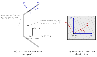

_images/vabs_axes.svg — (a) Axes \(x_1, x_2, x_3\) of a cross section, here a flared channel, with the local axes \(y_1, y_2, y_3\) of an element, oriented by `theta1`, and the tension and shear centres computed by `calc_stiffness()`; (b) the material axes \(m_1, m_2, m_3\) of the element, oriented by the ply angle `theta3`, see `rotate_material()`.#

Elements with 3, 4, 6, 8 and 9 nodes are supported: the linear and the quadratic triangles and the bilinear, serendipity and biquadratic quadrilaterals, with the nodes numbered counter-clockwise in the \(x_2 x_3\) plane, the corners first, then the mid-side nodes, starting with the one between the first two corners, then the centre node of the 9-node element. Different element types may be mixed when they share complete edges.

Parameters:

x2, x3array-like: Coordinates of the nodes, dimension length, 1-D arrays of size n_nodes.
elementssequence of sequences of int: Connectivity: for each element, the indices of its nodes in x2 and x3, starting at 0; size n_elements, each with 3, 4, 6, 8 or 9 indices.
materialssequence of array-like: Material matrices in the material axes, force per unit area, each of shape (6, 6) with the ordering of isotropic().
mat_idsarray-like: Index of the material of each element in materials, 1-D array of integers of size n_elements.
theta1array-like, optional: Angle of the local axes of each element, in degrees, 1-D array of size n_elements, see rotate_material(). Default None, meaning zero for all elements.
theta3array-like, optional: Ply angle of each element, in degrees, 1-D array of size n_elements, see rotate_material(). Default None, meaning zero for all elements.
densitiessequence of float, optional: Density of each material, mass per unit volume, size len(materials). Default None, meaning zero for all materials.
k1, k2, k3float, optional: Initial twist and initial curvatures of the beam, dimension inverse of length. Default 0., the only value implemented.

Attributes:

x2, x3np.ndarray: Coordinates of the nodes, dimension length.
connnp.ndarray: conn: object
nennp.ndarray: nen: object
mat_ids, theta1, theta3np.ndarray: As the parameters, size n_elements.
materialslist: materials: object
densitiesnp.ndarray: densities: object
Delnp.ndarray: Del: object
ndofint: ndof: ‘int’
constraintstr: constraint: object
areafloat: area: ‘double’
centroidnp.ndarray: centroid: object
Kcnp.ndarray: Kc: object
Fcnp.ndarray: Fc: object
Ktnp.ndarray: Kt: object
Ftnp.ndarray: Ft: object
tension_centrenp.ndarray: tension_centre: object
shear_centrenp.ndarray: shear_centre: object
V0np.ndarray: V0: object
V1Snp.ndarray: V1S: object
A, B, Cnp.ndarray: Matrices of the second-order energy, shape (4, 4), dimension of Kc times length to the power 0, 1 and 2.
Kvnp.ndarray: Kv: object
Fvnp.ndarray: Fv: object
vlasov_sectionCrossSection: vlasov_section: object
mass_per_lengthfloat: mass_per_length: ‘double’
mass_centrenp.ndarray: mass_centre: object
mass_matrixnp.ndarray: mass_matrix: object
intrho, intrhoy, intrhoz, intrhoy2, intrhoz2, intrhoyzfloat: Integrals of the density times \(1\), \(x_2\), \(x_3\), \(x_2^2\), \(x_3^2\) and \(x_2 x_3\), with the names of the attributes of BeamProp, where \(y = x_2\) and \(z = x_3\).

Methods

`calc_mass`(self)	Compute the mass properties of the cross section
`calc_stiffness`(self, str constraint=)	Compute the classical and generalized Timoshenko stiffnesses
`calc_vlasov`(self, str constraint=)	Compute the stiffness of the generalized Vlasov model
`translated`(self, double e2, double e3)	Copy of the cross section with the origin moved to a given point
`triangles`(self)	Linear triangles over all the nodes of the mesh, for plotting
`warping`(self, eps[, deps])	Nodal warping displacements for given beam strains

Raises:

NotImplementedError: If k1, k2 or k3 is not zero.
ValueError: If x2 and x3 have different sizes, if there is no element, if an element does not have 3, 4, 6, 8 or 9 nodes or refers to a node that does not exist, if a node is not used by any element, if a material matrix does not have the shape (6, 6), or if mat_ids, theta1, theta3 or densities do not have one entry per element or per material, or refer to a material that does not exist.

Notes

The cross-sectional analysis follows Cesnik and Hodges [1] and Yu et al. [2], see calc_stiffness() for the equations and _integrate() for the discretization.

References

[1]

[2]

Examples

A square of side 1 meshed with four bilinear quadrilaterals:

>>> import numpy as np
>>> from pyfe3d.vabs import CrossSection, isotropic
>>> x2, x3 = np.meshgrid([-0.5, 0., 0.5], [-0.5, 0., 0.5])
>>> elements = [[0, 1, 4, 3], [1, 2, 5, 4], [3, 4, 7, 6], [4, 5, 8, 7]]
>>> sec = CrossSection(x2.ravel(), x3.ravel(), elements,
...                    materials=[isotropic(1., 0.3)], mat_ids=[0]*4)
>>> sec.calc_stiffness()
>>> sec.Kt.shape
(6, 6)

A#: A: object

B#: B: object

C#: C: object

Del#: Del: object

Fc#: Fc: object

Ft#: Ft: object

Fv#: Fv: object

Kc#: Kc: object

Kt#: Kt: object

Kv#: Kv: object

V0#: V0: object

V1S#: V1S: object

area#: area: ‘double’

calc_mass(self)#

Compute the mass properties of the cross section

Integrates the densities of the materials over the cross section and sets mass_per_length, mass_centre, mass_matrix, intrho, intrhoy, intrhoz, intrhoy2, intrhoz2, intrhoyz, area and centroid. The mass centre is set to nan when the mass is zero.

Notes

The kinetic energy per unit length is Eq. (51) of [1], \(\mathcal{K} = \frac{1}{2} (\mu \boldsymbol{V}^\top \boldsymbol{V} + 2 \boldsymbol{\Omega}^\top \widetilde{\mu \bar{\xi}} \boldsymbol{V} + \boldsymbol{\Omega}^\top \boldsymbol{i} \boldsymbol{\Omega})\), with, Eq. (52) of [1], \(\mu = \langle \rho \rangle\), \(\mu \bar{\xi} = \langle \rho \xi \rangle\), \(\boldsymbol{i} = \langle \rho (\xi^\top \xi \boldsymbol{I} - \xi \xi^\top) \rangle\) and \(\xi = \{0, x_2, x_3\}\), where the tilde is the skew-symmetric matrix of the cross product. The mass matrix is then

\[\begin{split}\boldsymbol{M} = \begin{bmatrix} \mu \boldsymbol{I} & \widetilde{\mu \bar{\xi}}^\top \\ \widetilde{\mu \bar{\xi}} & \boldsymbol{i} \end{bmatrix}\end{split}\]

References

[1] (1,2)

calc_stiffness(self, str constraint='yu2012')#

Compute the classical and generalized Timoshenko stiffnesses

Assembles the matrices of the cross section, solves the warping problems of the classical model and of its refinement with one sparse LU factorization, and sets Kc, Fc, Kt, Ft, tension_centre, shear_centre, V0, V1S, A, B, C, constraint, area and centroid. The tension centre is the point where an axial force gives no bending curvature, and the shear centre the point where a transverse force gives no twist, see the figure of CrossSection.

Parameters:

constraintstr, optional: The four constraints that make the warping unique: 'yu2012', the default, zero average warping and zero average rotation of the warping, or 'yu2002', zero average warping and zero average of \(x_2 w_3 - x_3 w_2\). They change V0 and the Timoshenko matrices, not Kc.

Raises:

ValueError: If constraint is not one of the above, or if an element has a non-positive Jacobian determinant, e.g. when its nodes are numbered clockwise.
RuntimeError: If the mesh is not connected, or if the constrained warping problem is otherwise singular.

Notes

Classical model. With the matrices of _integrate(), the energy per unit length of a prismatic beam without the terms in the derivatives of the warping is, Eq. (75) of [1],

\[2 \mathcal{U}_0 = \boldsymbol{V}^\top \boldsymbol{D}_{hh} \boldsymbol{V} + 2 \boldsymbol{V}^\top \boldsymbol{D}_{h\epsilon} \bar{\boldsymbol{\epsilon}} + \bar{\boldsymbol{\epsilon}}^\top \boldsymbol{D}_{\epsilon\epsilon} \bar{\boldsymbol{\epsilon}}\]

and its minimum subject to the constraints \(\boldsymbol{D}_c^\top \boldsymbol{V} = \boldsymbol{0}\), Eqs. (78)–(85) of [1], is \(\boldsymbol{V}_0 = \hat{\boldsymbol{V}}_0 \bar{\boldsymbol{\epsilon}}\) (V0), from the system with the Lagrange multipliers \(\boldsymbol{\Lambda}\)

\[\begin{split}\begin{bmatrix} \boldsymbol{D}_{hh} & \boldsymbol{D}_c \\ \boldsymbol{D}_c^\top & \boldsymbol{0} \end{bmatrix} \begin{Bmatrix} \hat{\boldsymbol{V}}_0 \\ \boldsymbol{\Lambda} \end{Bmatrix} = \begin{Bmatrix} -\boldsymbol{D}_{h\epsilon} \\ \boldsymbol{0} \end{Bmatrix}\end{split}\]

which is regular because \(\boldsymbol{D}_c^\top \boldsymbol{\Psi}\) is regular, \(\boldsymbol{\Psi}\) being the four rigid-body modes of the kernel of \(\boldsymbol{D}_{hh}\), Eq. (41) of [1]. The multipliers vanish for this right-hand side, which is orthogonal to \(\boldsymbol{\Psi}\), Eq. (81) of [1], and the constraints do not change the classical stiffness, Eq. (86) of [1],

\[\boldsymbol{A} = \hat{\boldsymbol{V}}_0^\top \boldsymbol{D}_{h\epsilon} + \boldsymbol{D}_{\epsilon\epsilon}\]

stored in Kc and A.

Refinement. With \(\boldsymbol{V} = \boldsymbol{V}_0 + \boldsymbol{V}_1\) and the terms in \(\boldsymbol{V}'\), the first-order warping of a prismatic beam is \(\boldsymbol{V}_1 = \hat{\boldsymbol{V}}_{1S} \bar{\boldsymbol{\epsilon}}'\) (V1S), Eqs. (96)–(101) of [1] with \(\boldsymbol{D}_R = \boldsymbol{0}\), no applied loads, and

\[\boldsymbol{D}_S = (\boldsymbol{D}_{hl} - \boldsymbol{D}_{hl}^\top) \hat{\boldsymbol{V}}_0 - \boldsymbol{D}_{l\epsilon}\]

solved from the same system with \(-\boldsymbol{D}_S\) on the right-hand side, whose multipliers do not vanish, Eq. (100) of [1]. The second-order energy is \(2\mathcal{U} = \bar{\boldsymbol{\epsilon}}^\top \boldsymbol{A} \bar{\boldsymbol{\epsilon}} + 2 \bar{\boldsymbol{\epsilon}}^\top \boldsymbol{B} \bar{\boldsymbol{\epsilon}}' + \bar{\boldsymbol{\epsilon}}'^\top \boldsymbol{C} \bar{\boldsymbol{\epsilon}}' + 2 \bar{\boldsymbol{\epsilon}}^\top \boldsymbol{D} \bar{\boldsymbol{\epsilon}}''\), Eqs. (102) and (103) of [1] with the initial curvatures set to zero,

\[\boldsymbol{B} = \hat{\boldsymbol{V}}_0^\top \boldsymbol{D}_{hl} \hat{\boldsymbol{V}}_0 + \boldsymbol{D}_{l\epsilon}^\top \hat{\boldsymbol{V}}_0 \qquad \boldsymbol{C} = \hat{\boldsymbol{V}}_{1S}^\top \bar{\boldsymbol{D}}_S + \hat{\boldsymbol{V}}_0^\top \boldsymbol{D}_{ll} \hat{\boldsymbol{V}}_0 \qquad \bar{\boldsymbol{D}}_S = (\boldsymbol{D}_{hl} + \boldsymbol{D}_{hl}^\top) \hat{\boldsymbol{V}}_0 + \boldsymbol{D}_{l\epsilon}\]

where \(\boldsymbol{C}\) is stored symmetrized; \(\boldsymbol{D}\) does not enter the stiffness of a prismatic beam.

Transformation to the generalized Timoshenko form. For a prismatic beam, the energy \(2\mathcal{U} = \boldsymbol{\epsilon}^\top \boldsymbol{X} \boldsymbol{\epsilon} + 2 \boldsymbol{\epsilon}^\top \boldsymbol{Y} \boldsymbol{\gamma}_s + \boldsymbol{\gamma}_s^\top \boldsymbol{G} \boldsymbol{\gamma}_s\), with \(\boldsymbol{\gamma}_s = \{2\gamma_{12}, 2\gamma_{13}\}\), is obtained in closed form, Eqs. (105)–(107) of [1], as

\[\boldsymbol{G} = \left[ \boldsymbol{Q}^\top \boldsymbol{A}^{-1} (\boldsymbol{C} - \boldsymbol{B}^\top \boldsymbol{A}^{-1} \boldsymbol{B}) \boldsymbol{A}^{-1} \boldsymbol{Q} \right]^{-1} \qquad \boldsymbol{Y} = \boldsymbol{B}^\top \boldsymbol{A}^{-1} \boldsymbol{Q} \boldsymbol{G} \qquad \boldsymbol{X} = \boldsymbol{A} + \boldsymbol{Y} \boldsymbol{G}^{-1} \boldsymbol{Y}^\top\]

with \(\boldsymbol{Q}\) of Eq. (28) of [1], rows \(\{0, 0\}\), \(\{0, 0\}\), \(\{0, -1\}\), \(\{1, 0\}\), which follows from the kinematic relation between the classical and the Timoshenko strains, Eq. (27) of [1], and from the one-dimensional equilibrium equations. The matrix Kt is \([\boldsymbol{X}, \boldsymbol{Y}; \boldsymbol{Y}^\top, \boldsymbol{G}]\) reordered to interleave the shear strains, as in Eq. (109) of [1]. By construction the classical stiffness obtained from the Timoshenko flexibility by deleting the shear rows and columns and inverting, as prescribed on p. 52 of [2], is Kc.

Centres. The shear centre is Eq. (66) of [3], \(e_2 = -P_{34} / P_{44}\), \(e_3 = P_{24}/P_{44}\), with \(P_{ij}\) the entries of Ft numbered from 1. The tension centre \((a_2, a_3)\) is the point where an axial force \(F_1\), with the moments \(M_2 = a_3 F_1\) and \(M_3 = -a_2 F_1\) about the reference axis, gives \(\kappa_2 = \kappa_3 = 0\) through Fc, a definition of this module.

References

[1] (1,2,3,4,5,6,7,8,9,10,11,12)

[2]

[3]

calc_vlasov(self, str constraint='yu2002')#

Compute the stiffness of the generalized Vlasov model

Locates the shear centre, analyses with calc_stiffness() the cross section translated to it, stored in vlasov_section, and sets Kv and Fv, the \(5 \times 5\) stiffness and flexibility of the strains \(\{\gamma_{11}, \kappa_1, \kappa_2, \kappa_3, \kappa_1'\}\) referred to the shear centre, where \(\kappa_1'\) is the derivative of the twist rate along the beam and the bimoment \(M_\omega\) its work-conjugate. The model is intended for thin-walled open sections, whose restrained warping is not represented by the classical and Timoshenko models. The other attributes are not changed. No beam element of pyfe3d uses Kv: BeamC and BeamLR have no warping degree-of-freedom, and Kv is meant for one-dimensional Vlasov beam analyses outside pyfe3d.

Parameters:

constraintstr, optional: The warping constraints of calc_stiffness(). Default 'yu2002', with which the published values of the generalized Vlasov model are reproduced, see the Notes. 'yu2012', the default of calc_stiffness(), gives the same first four rows and columns and, in the tested cases, the same shear centre, but a different warping rigidity Kv[4, 4]: lower by up to about 12 per cent for a strip, and by about 0.1 per cent for I- and channel sections.

Raises:

ValueError: As calc_stiffness().
RuntimeError: As calc_stiffness().

Notes

The second-order energy of a prismatic beam, \(2\mathcal{U} = \bar{\boldsymbol{\epsilon}}^\top \boldsymbol{A} \bar{\boldsymbol{\epsilon}} + 2 \bar{\boldsymbol{\epsilon}}^\top \boldsymbol{B} \bar{\boldsymbol{\epsilon}}' + \bar{\boldsymbol{\epsilon}}'^\top \boldsymbol{C} \bar{\boldsymbol{\epsilon}}' + 2 \bar{\boldsymbol{\epsilon}}^\top \boldsymbol{D} \bar{\boldsymbol{\epsilon}}''\), Eq. (1) of [1], see calc_stiffness(), depends on the reference axis. Following Section 2 of [1], the shear centre is obtained from the generalized Timoshenko flexibility, Eq. (3) of [1], shear_centre, the origin is moved to it, and only the derivative \(\kappa_1'\) of the twist rate is kept, \(\gamma_{11}' = \kappa_2' = \kappa_3' = 0\), which gives the generalized Vlasov model, Eq. (4) of [1],

\[\begin{split}\boldsymbol{K}_v = \begin{bmatrix} \boldsymbol{A} & \boldsymbol{b} \\ \boldsymbol{b}^\top & C_{22} \end{bmatrix} \qquad \boldsymbol{b} = \{B_{12}, B_{22}, B_{32}, B_{42}\}\end{split}\]

with \(\boldsymbol{A}\), \(\boldsymbol{B}\) and \(\boldsymbol{C}\) those of the translated section and the entries numbered from 1. The first four rows and columns are the classical stiffness in the axes of the shear centre. The term in \(\boldsymbol{D}\) contains \(\kappa_1''\) and has no place in Eq. (4) of [1]; it is omitted, as in [1], whose values are reproduced without it.

The two sets of warping constraints differ in the fourth one, on the rotation of the in-plane warping. This changes \(\boldsymbol{C}\), hence \(K_{v,55}\), but not \(\boldsymbol{A}\) and \(\boldsymbol{B}\). With the constraints of Yu et al. (2002), constraint='yu2002', \(K_{v,55}\) reproduces the values computed with VABS in Tables 1, 3 and 4 of [1] for strips to five digits or more, and for the isotropic strip it agrees with the asymptotic thin-walled value \(E h^3 b^3/[144 (1 - \nu^2)]\), Eq. (18) of [1]. With constraint='yu2012' it is lower for the strips, by \(9.5\) per cent for the isotropic one, close to the value \(E h^3 b^3/144\) of Vlasov’s theory, Eq. (17) of [1], by \(1.9\) per cent for the orthotropic one and by \(12\) per cent for the anisotropic one of Table 4 of [1]. For I- and channel sections, the two are within about \(0.1\) per cent of each other and within \(0.4\) per cent of the thin-walled warping rigidity. Since only 'yu2002' reproduces [1], it is the default.

For a thin-walled open section, the torsional warping per unit twist rate about the shear centre, the first column of vlasov_section.warping([0, 1, 0, 0]), approaches \(-\omega\), with \(\omega\) the principal sectorial coordinate of Vlasov [2], Eqs. (3.15) and (7.1), pp. 14–16 and 40–41, normalised to zero average with the pole at the shear centre, Sec. 9, pp. 51–53, and \(K_{v,55}\) approaches the warping rigidity \(E \Gamma\).

References

[1] (1,2,3,4,5,6,7,8,9,10,11)

[2]

Vlasov, V. Z., Thin-Walled Elastic Beams, 2nd ed., Israel Program for Scientific Translations, Jerusalem, 1961. Translated by Y. Schechtman.

Examples

Warping rigidity of a thin-walled I-section, flanges of width 1 and walls of thickness 0.04, outer height 0.5, close to \(E t b_f^3 h^2/24\) with \(h = 0.46\) between the flange mid-planes:

>>> import numpy as np
>>> from pyfe3d.vabs import CrossSection, isotropic
>>> t, H, w = 0.04, 0.5, 0.48
>>> def rect(a, b, nx, ny, x0, y0):
...     x2, x3 = np.meshgrid(x0 + np.linspace(-a/2, a/2, nx + 1),
...                          y0 + np.linspace(-b/2, b/2, ny + 1))
...     els = [[j*(nx + 1) + i, j*(nx + 1) + i + 1,
...             (j + 1)*(nx + 1) + i + 1, (j + 1)*(nx + 1) + i]
...            for j in range(ny) for i in range(nx)]
...     return x2.ravel(), x3.ravel(), els
>>> parts = [rect(w, t, 12, 2, -t/2 - w/2, y) for y in (-0.23, 0.23)]
>>> parts += [rect(w, t, 12, 2, t/2 + w/2, y) for y in (-0.23, 0.23)]
>>> parts += [rect(t, t, 2, 2, 0., y) for y in (-0.23, 0.23)]
>>> parts += [rect(t, H - 2*t, 2, 10, 0., 0.)]
>>> xy = np.round(np.concatenate([np.column_stack(p[:2])
...                               for p in parts]), 9)
>>> uniq, inv = np.unique(xy, axis=0, return_inverse=True)
>>> inv = inv.ravel()
>>> offsets = np.cumsum([0] + [len(p[0]) for p in parts])
>>> elements = [[int(inv[o + n]) for n in el]
...             for p, o in zip(parts, offsets) for el in p[2]]
>>> sec = CrossSection(uniq[:, 0], uniq[:, 1], elements,
...                    materials=[isotropic(10e6, 0.3)],
...                    mat_ids=[0]*len(elements))
>>> sec.calc_vlasov()
>>> EG = 10e6*t*1.**3*0.46**2/24
>>> bool(abs(sec.Kv[4, 4]/EG - 1) < 0.01)
True

centroid#: centroid: object

conn#: conn: object

constraint#: constraint: object

densities#: densities: object

intrho#: intrho: ‘double’

intrhoy#: intrhoy: ‘double’

intrhoy2#: intrhoy2: ‘double’

intrhoyz#: intrhoyz: ‘double’

intrhoz#: intrhoz: ‘double’

intrhoz2#: intrhoz2: ‘double’

mass_centre#: mass_centre: object

mass_matrix#: mass_matrix: object

mass_per_length#: mass_per_length: ‘double’

mat_ids#: mat_ids: object

materials#: materials: object

ndof#: ndof: ‘int’

nen#: nen: object

shear_centre#: shear_centre: object

tension_centre#: tension_centre: object

theta1#: theta1: object

theta3#: theta3: object

translated(self, double e2, double e3)#

Copy of the cross section with the origin moved to a given point

Creates a new CrossSection with the same mesh, materials, orientations and densities, whose coordinates are \(x_2 - e_2\) and \(x_3 - e_3\), i.e. whose reference axis passes through the point \((e_2, e_3)\) of this cross section. Nothing is computed.

Parameters:

e2, e3float: Coordinates of the new origin in the axes of this cross section, dimension length, e.g. *shear_centre.

Returns:

secCrossSection: The translated cross section.

Examples

>>> import numpy as np
>>> from pyfe3d.vabs import CrossSection, isotropic
>>> x2, x3 = np.meshgrid([-0.5, 0., 0.5], [-0.5, 0., 0.5])
>>> elements = [[0, 1, 4, 3], [1, 2, 5, 4], [3, 4, 7, 6], [4, 5, 8, 7]]
>>> sec = CrossSection(x2.ravel(), x3.ravel(), elements,
...                    materials=[isotropic(1., 0.3)], mat_ids=[0]*4)
>>> float(sec.translated(0.5, 0.).x2.min())
-1.0

triangles(self)#

Linear triangles over all the nodes of the mesh, for plotting

Splits every element into 3-node triangles whose vertices are its nodes, counter-clockwise, such that a field given at the nodes, e.g. a column of warping(), can be drawn with any plotting library that accepts a triangulation. The bilinear quadrilateral gives two triangles; the 6-node triangle four, through its mid-side nodes; the 9-node quadrilateral eight, two for each quarter around the centre node; and the 8-node quadrilateral six, one at each corner, cut through the two adjacent mid-side nodes, and two for the quadrilateral of the four mid-side nodes.

Returns:

trinp.ndarray: Node indices of the triangles, shape (n_triangles, 3).

Examples

>>> import numpy as np
>>> from pyfe3d.vabs import CrossSection, isotropic
>>> x2, x3 = np.meshgrid([-0.5, 0., 0.5], [-0.5, 0., 0.5])
>>> elements = [[0, 1, 4, 3], [1, 2, 5, 4], [3, 4, 7, 6], [4, 5, 8, 7]]
>>> sec = CrossSection(x2.ravel(), x3.ravel(), elements,
...                    materials=[isotropic(1., 0.3)], mat_ids=[0]*4)
>>> sec.triangles().shape
(8, 3)

vlasov_section#: vlasov_section: object

warping(self, eps, deps=None, str convention='yu')#

Nodal warping displacements for given beam strains

Combines the warping per unit strain stored by calc_stiffness(), V0 for the classical strains and V1S for their derivatives along the beam, into the warping displacements \(w_1, w_2, w_3\) of every node, e.g. to plot the warping of a cross section with triangles().

Parameters:

epsarray-like: Classical strains, size 4: \(\{\gamma_{11}, \kappa_1, \kappa_2, \kappa_3\}\) for convention='yu', or \(\{\bar{\varepsilon}, \kappa_x, \kappa_y, \kappa_z\}\) for convention='pyfe3d', see yu_to_pyfe3d(); dimension inverse of length for the curvatures.
depsarray-like, optional: Derivatives of the classical strains along the beam axis \(x_1\), size 4, same convention as eps. Default None, meaning zero, i.e. without the warping of the transverse shear of the generalized Timoshenko model.
conventionstr, optional: 'yu', the default, or 'pyfe3d'.

Returns:

wnp.ndarray: Warping displacements \(w_1, w_2, w_3\) of each node, shape (n_nodes, 3), dimension length; \(w_1\) is along the beam axis and \(w_2\), \(w_3\) in the plane of the cross section.

Raises:

RuntimeError: If calc_stiffness() has not been called.
ValueError: If eps or deps does not have size 4, or if convention is not 'yu' or 'pyfe3d'.

Examples

Torsional warping per unit twist rate \(\kappa_1 = 1\) of a rectangle, which is antisymmetric about both axes:

>>> import numpy as np
>>> from pyfe3d.vabs import CrossSection, isotropic
>>> x2, x3 = np.meshgrid([-1., 0., 1.], [-0.25, 0., 0.25])
>>> elements = [[0, 1, 4, 3], [1, 2, 5, 4], [3, 4, 7, 6], [4, 5, 8, 7]]
>>> sec = CrossSection(x2.ravel(), x3.ravel(), elements,
...                    materials=[isotropic(1., 0.3)], mat_ids=[0]*4)
>>> sec.calc_stiffness()
>>> w = sec.warping([0., 1., 0., 0.])
>>> w.shape
(9, 3)
>>> bool(np.isclose(w[0, 0], -w[2, 0]))
True

x2#: x2: object

x3#: x3: object

pyfe3d.vabs.beamprop_from_vabs(Cs, double E, CrossSection sec=None)#

Create a BeamProp from a sectional stiffness matrix

The sectional stiffness matrix C of the property, read by the beam elements of pyfe3d, is set to Cs, with all its 21 independent entries, couplings included. The 11 stiffness attributes of the property, which the elements do not read once C is set, are also filled from the entries of Cs of the pattern given in the notes of BeamProp, for information: the integrals of the cross section are modulus-weighted, A is Cs[0, 0]/E, Iyy is Cs[5, 5]/E, etc., with G12, G13 and GJ read from the shear and torsion entries.

Parameters:

Csarray-like: Generalized Timoshenko stiffness matrix in the convention of pyfe3d, e.g. yu_to_pyfe3d(sec.Kt), shape (6, 6), symmetric, see BeamProp for the order of the strains.
Efloat: Reference Young modulus stored in E of the property and used for the modulus-weighted attributes, force per unit area.
secCrossSection, optional: When given, the mass integrals intrho, intrhoy, intrhoz, intrhoy2, intrhoz2 and intrhoyz are copied from it, so CrossSection.calc_mass() must have been called. Default None, leaving them equal to zero.

Returns:

propBeamProp: The property, with C equal to Cs, the attributes A, E, G12, G13, GJ, Ay, Az, Iyy, Izz and Iyz and, optionally, the mass integrals set.

Raises:

ValueError: If Cs does not have the shape (6, 6) or is not symmetric, or if E or Cs[0, 0] is not positive.

Notes

A composite section generally has couplings that the 11 attributes cannot represent, e.g. the extension-twist coupling Cs[0, 3] and the bending-shear couplings Cs[1, 5] and Cs[2, 4] of the CUS box of Yu et al. [1], Table 2. They are kept in C; del prop.C returns to the property of the 11 attributes, which drops them. The accuracy of BeamC and BeamLR with a coupled matrix is discussed in the notes of BeamC.

References

[1]

Examples

>>> import numpy as np
>>> from pyfe3d.vabs import beamprop_from_vabs
>>> Cs = np.diag([7e9, 2e9, 2e9, 1e6, 6e6, 6e6])
>>> Cs[0, 3] = Cs[3, 0] = 1e6
>>> prop = beamprop_from_vabs(Cs, E=70e9)
>>> prop.A
0.1
>>> prop.C[0, 3]
1000000.0

pyfe3d.vabs.classical_from_timoshenko(Kt)#

Classical stiffness matrix from a generalized Timoshenko one

Inverts the \(6 \times 6\) stiffness, deletes the rows and columns of the two transverse shear strains from the flexibility, and inverts the remaining \(4 \times 4\) matrix.

Parameters:

Ktarray-like: Generalized Timoshenko stiffness matrix in the convention of this module, shape (6, 6).

Returns:

Kcnp.ndarray: Classical stiffness matrix of \(\{\gamma_{11}, \kappa_1, \kappa_2, \kappa_3\}\), shape (4, 4).

Raises:

ValueError: If Kt does not have the shape (6, 6).

Notes

This is the reduction prescribed on p. 52 of Yu and Hodges [1], a static condensation of the shear strains under zero shear forces. For the prismatic beams of CrossSection it returns Kc, see CrossSection.calc_stiffness().

References

[1]

Examples

>>> import numpy as np
>>> from pyfe3d.vabs import classical_from_timoshenko
>>> Kc = classical_from_timoshenko(np.diag([1., 2., 3., 4., 5., 6.]))
>>> np.diag(Kc)
array([1., 4., 5., 6.])

pyfe3d.vabs.isotropic(double E, double nu)#

Material matrix of an isotropic material

Parameters:

Efloat: Young modulus, force per unit area.
nufloat: Poisson ratio, dimensionless.

Returns:

Dnp.ndarray: Material matrix, force per unit area, shape (6, 6), relating the stresses \(\{\sigma_{11}, \sigma_{12}, \sigma_{13}, \sigma_{22}, \sigma_{23}, \sigma_{33}\}\) to the strains \(\{\Gamma_{11}, 2\Gamma_{12}, 2\Gamma_{13}, \Gamma_{22}, 2\Gamma_{23}, \Gamma_{33}\}\), the ordering used by CrossSection.

Raises:

ValueError: If E is not positive or nu is not between -1 and 0.5, both excluded.

Examples

>>> from pyfe3d.vabs import isotropic
>>> D = isotropic(E=70e9, nu=0.3)
>>> D.shape
(6, 6)

pyfe3d.vabs.orthotropic(double E1, double E2, double E3, double G12, double G13, double G23, double nu12, double nu13, double nu23)#

Material matrix of an orthotropic material in its material axes

Parameters:

E1, E2, E3float: Young moduli along the material axes \(1\), \(2\) and \(3\), force per unit area.
G12, G13, G23float: Shear moduli of the planes \(12\), \(13\) and \(23\), force per unit area.
nu12, nu13, nu23float: Poisson ratios, dimensionless, with nu12 the contraction along \(2\) for a tension along \(1\), and likewise for nu13 and nu23.

Returns:

Dnp.ndarray: Material matrix in the material axes, force per unit area, shape (6, 6), with the ordering of isotropic().

Raises:

ValueError: If the matrix is not positive definite.

Examples

>>> from pyfe3d.vabs import orthotropic
>>> D = orthotropic(E1=20.59e6, E2=1.42e6, E3=1.42e6, G12=0.87e6,
...                 G13=0.87e6, G23=0.696e6, nu12=0.30, nu13=0.30,
...                 nu23=0.34)
>>> D.shape
(6, 6)

pyfe3d.vabs.pyfe3d_to_yu(Cs, double h=1.)#

Convert a sectional matrix from the convention of pyfe3d to that of this module

Inverse of yu_to_pyfe3d().

Parameters:

Csarray-like: Stiffness matrix in the convention of pyfe3d, shape (6, 6) or (4, 4).
hfloat, optional: As in yu_to_pyfe3d(), dimension length. Default 1..

Returns:

Cnp.ndarray: Stiffness matrix in the convention of this module, same shape as Cs.

Raises:

ValueError: If Cs does not have the shape (6, 6) or (4, 4).

Variational asymptotic sectional analysis (pyfe3d.vabs)#

Notes#

References#

Variational asymptotic sectional analysis (`pyfe3d.vabs`)#