Natural frequency analysis of a cylinder#
The figure below shows the first vibration mode of a cylindrical shell with CC2
boundary conditions. The figure was generated using refinement=2 and
running the script directly.
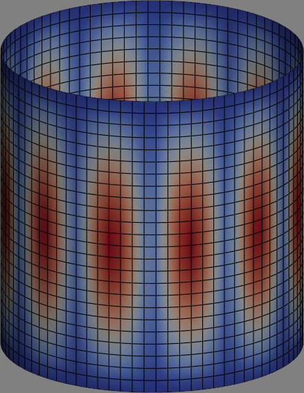
The code used to generate this figure is extracted from one of pyfe3d unit
tests:
import sys
sys.path.append('..')

import time
import numpy as np
from numpy import isclose
from scipy.sparse import coo_matrix

from pyfe3d.shellprop_utils import laminated_plate
from pyfe3d import Quad4, Quad4Data, Quad4Probe, INT, DOUBLE, DOF
from pyfe3d.solver import natural_frequency


def test_linear_nat_freq_cylinder(mode=0, plot_pyvista=False, refinement=1):
    r"""Test case from reference

        Saullo G. P. Castro, Christian Mittelstedt, Francisco A. C. Monteiro, Mariano
        A. Arbelo, Gerhard Ziegmann, Richard Degenhardt. "Linear buckling predictions
        of unstiffened laminated composite cylinders and cones under various loading
        and boundary conditions using semi-analytical models". Composite Structures,
        2014. 10.1016/j.compstruct.2014.07.037

        Cylinders Z11

    """
    data = Quad4Data()
    probe = Quad4Probe()

    L = 0.510 # m
    R = 0.250 # m
    b = 2*np.pi*R # m

    ntheta = 40*refinement # circumferential
    nlength = int(ntheta*L/b)
    if nlength % 2 == 0:
        nlength += 1
    print('ntheta', ntheta)
    print('nlength', nlength)

    # NOTE material proporties from Table 3 in Castro et al.
    # Actual values from reference can be found here https://github.com/saullocastro/compmech/blob/e7e5342bf212743e70da22c94cc0452911099db3/compmech/conecyl/conecylDB.py#L32C34-L32C76
    E11 = 123.55e9
    E22 = 8.7079e9
    nu12 = 0.319
    G12 = 5.696e9
    G13 = 5.696e9
    G23 = 3.400e9
    plyt = 0.125e-3
    rho = 1.78e3 # kg/m3
    laminaprop = (E11, E22, nu12, G12, G13, G23)

    # NOTE cylinder Z11, Table 4 of Castro et al., Table 3 being the one
    #      with the material properties
    # NOTE the reference is the source of the geometry, the material and the
    #      stacking sequence only. It is a linear buckling paper: it contains
    #      no natural frequencies, and no density either, so the value of rho
    #      above does not come from it. The frequencies asserted at the end
    #      of this test are recorded pyfe3d output and are a regression lock,
    #      not a comparison with the literature
    stack = [+60, -60, 0, 0, +68, -68, +52, -52, +37, -37]
    prop = laminated_plate(stack=stack, plyt=plyt, laminaprop=laminaprop,
                           rho=rho)

    nids = 1 + np.arange(nlength*(ntheta+1))
    nids_mesh = nids.reshape(nlength, ntheta+1)
    nids_mesh[:, -1] = nids_mesh[:, 0]
    nids = np.unique(nids_mesh)
    nid_pos = dict(zip(nids, np.arange(len(nids))))

    zlin = np.linspace(0, L, nlength)
    thetatmp = np.linspace(0, 2*np.pi, ntheta+1)
    thetalin = np.linspace(0, 2*np.pi-(thetatmp[-1] - thetatmp[-2]), ntheta)[::-1]
    zmesh, thetamesh = np.meshgrid(zlin, thetalin)
    zmesh = zmesh.T
    thetamesh = thetamesh.T
    xmesh = np.cos(thetamesh)*R
    ymesh = np.sin(thetamesh)*R

    ncoords = np.vstack((xmesh.flatten(), ymesh.flatten(), zmesh.flatten())).T
    ncoords_flatten = ncoords.flatten()
    x = ncoords[:, 0]
    y = ncoords[:, 1]
    z = ncoords[:, 2]

    n1s = nids_mesh[:-1, :-1].flatten()
    n2s = nids_mesh[1:, :-1].flatten()
    n3s = nids_mesh[1:, 1:].flatten()
    n4s = nids_mesh[:-1, 1:].flatten()

    num_elements = len(n1s)
    print('num_elements', num_elements)

    KC0r = np.zeros(data.KC0_SPARSE_SIZE*num_elements, dtype=INT)
    KC0c = np.zeros(data.KC0_SPARSE_SIZE*num_elements, dtype=INT)
    KC0v = np.zeros(data.KC0_SPARSE_SIZE*num_elements, dtype=DOUBLE)
    Mr = np.zeros(data.M_SPARSE_SIZE*num_elements, dtype=INT)
    Mc = np.zeros(data.M_SPARSE_SIZE*num_elements, dtype=INT)
    Mv = np.zeros(data.M_SPARSE_SIZE*num_elements, dtype=DOUBLE)
    N = DOF*nlength*ntheta

    quads = []
    init_k_KC0 = 0
    init_k_M = 0
    t0 = time.time()
    for n1, n2, n3, n4 in zip(n1s, n2s, n3s, n4s):
        quad = Quad4(probe)
        quad.n1 = n1
        quad.n2 = n2
        quad.n3 = n3
        quad.n4 = n4
        quad.c1 = DOF*nid_pos[n1]
        quad.c2 = DOF*nid_pos[n2]
        quad.c3 = DOF*nid_pos[n3]
        quad.c4 = DOF*nid_pos[n4]
        quad.init_k_KC0 = init_k_KC0
        quad.init_k_M = init_k_M
        quad.K6ROT = 100.
        quad.update_rotation_matrix(ncoords_flatten, 0., 0., 1.)
        quad.update_probe_xe(ncoords_flatten)
        quad.update_KC0(KC0r, KC0c, KC0v, prop)
        quad.update_M(Mr, Mc, Mv, prop, mtype=0) # consistent mass
        quads.append(quad)
        init_k_KC0 += data.KC0_SPARSE_SIZE
        init_k_M += data.M_SPARSE_SIZE

    print('elements created', time.time()-t0)

    KC0 = coo_matrix((KC0v, (KC0r, KC0c)), shape=(N, N)).tocsc()
    M = coo_matrix((Mv, (Mr, Mc)), shape=(N, N)).tocsc()

    print('sparse KC0 and M created')

    bk = np.zeros(N, dtype=bool)

    # NOTE cylinders with CC2 boundary condition as decribed in Table 1 of Castro et al.
    bottom_edge = isclose(z, 0)
    bk[0::DOF][bottom_edge] = True
    bk[1::DOF][bottom_edge] = True
    bk[3::DOF][bottom_edge] = True
    bk[4::DOF][bottom_edge] = True

    top_edge = isclose(z, L)
    bk[0::DOF][top_edge] = True
    bk[1::DOF][top_edge] = True
    bk[3::DOF][top_edge] = True
    bk[4::DOF][top_edge] = True

    middle = isclose(z, L/2)
    bk[2::DOF][middle] = True

    bu = ~bk

    KC0uu = KC0[bu, :][:, bu]
    Muu = M[bu, :][:, bu]

    num_eig = max(mode+1, 6)

    eigvecs = np.zeros((N, num_eig))

    # NOTE pyfe3d.solver.natural_frequency equilibrates the diagonal
    #      before calling the eigensolver and returns the circular
    #      frequencies already sorted
    omegan, eigvecsu = natural_frequency(KC0uu, Muu, num_eigvalues=num_eig, tol=1e-6)

    eigvecs[bu] = eigvecsu


    print('natural frequency analysis OK')

    print('omegan =', omegan)

    if plot_pyvista:
        import pyvista as pv

        contour_colorscale = 'coolwarm'
        background = 'gray'
        contour_label = 'Radial displacement'
        vector = eigvecs[:, mode]
        contour_vec = np.sqrt(vector[0::DOF]**2 + vector[1::DOF]**2)
        displ_vec = np.zeros_like(ncoords)
        displ_vec[:, 0] = vector[0::DOF]*10
        displ_vec[:, 1] = vector[1::DOF]*10
        displ_vec[:, 2] = vector[2::DOF]*10
        intensitymode = 'vertex'

        plotter = pv.Plotter(off_screen=False)
        faces_quad = []
        for q in quads:
            faces_quad.append([4, nid_pos[q.n1], nid_pos[q.n2], nid_pos[q.n3], nid_pos[q.n4]])
        faces_quad = np.array(faces_quad)
        quad_plot = pv.PolyData(ncoords, faces_quad)
        if contour_vec is not None:
            quad_plot[contour_label] = contour_vec
            plotter.add_mesh(quad_plot, scalars=contour_label,
                    cmap=contour_colorscale, edge_color='black', show_edges=True,
                    line_width=1.)
        else:
            plotter.add_mesh(quad_plot, edge_color='black', show_edges=True,
                    line_width=1.)
        displ_vec = None
        if displ_vec is not None:
            quad_plot = pv.PolyData(ncoords + displ_vec, faces_quad)
            plotter.add_mesh(quad_plot, edge_color='red', show_edges=True,
                    line_width=1., opacity=0.5)
        #NOTE plotting coordinate system
        xaxis = pv.Arrow(start=(0, 0, 0), direction=(1, 0, 0), scale=R/3)
        plotter.add_mesh(xaxis, color='blue')
        yaxis = pv.Arrow(start=(0, 0, 0), direction=(0, 1, 0), scale=R/3)
        plotter.add_mesh(yaxis, color='yellow')
        zaxis = pv.Arrow(start=(0, 0, 0), direction=(0, 0, 1), scale=R/3)
        plotter.add_mesh(zaxis, color='green')

        if False:
            for q in quads:
                pos1 = nid_pos[q.n1]
                pos2 = nid_pos[q.n2]
                pos3 = nid_pos[q.n3]
                pos4 = nid_pos[q.n4]
                centroid = (ncoords[pos1] + ncoords[pos2] + ncoords[pos3] + ncoords[pos4])/4
                ze = np.array([0., 0., 1.])
                zg = np.array([[q.r11, q.r12, q.r13],
                               [q.r21, q.r22, q.r23],
                               [q.r31, q.r32, q.r33]]) @ ze
                normal = pv.Arrow(start=centroid, direction=zg, scale=R/6)
                plotter.add_mesh(normal, color='green')

                xe = np.array([1., 0., 0.])
                xg = np.array([[q.r11, q.r12, q.r13],
                               [q.r21, q.r22, q.r23],
                               [q.r31, q.r32, q.r33]]) @ xe
                x_axis = pv.Arrow(start=centroid, direction=xg, scale=R/6)
                plotter.add_mesh(x_axis, color='blue')

                ye = np.array([0., 1., 0.])
                yg = np.array([[q.r11, q.r12, q.r13],
                               [q.r21, q.r22, q.r23],
                               [q.r31, q.r32, q.r33]]) @ ye
                y_axis = pv.Arrow(start=centroid, direction=yg, scale=R/6)
                plotter.add_mesh(y_axis, color='yellow')

        plotter.set_background(background)
        plotter.parallel_projection = True
        plotter.show()

    # NOTE reference values updated after adopting the equilibrium-based
    #      transverse shear stiffness of Rohwer (1988), evaluated in the element
    #      frame, which changed them by about 1e-4
    # NOTE reference values updated again in 0.10.0, when the physics-based
    #      drilling stiffness of Allman, Hughes and Brezzi became the default.
    #      Two changes contribute. First, the drilling penalty coefficient
    #      K6ROT*1e-6*A66 was restored (it had been lost, leaving an effective
    #      coefficient of 1), which by itself moves the frequencies from
    #      [1932.79, 2105.30, 2114.87] to [1958.18, 2115.51, 2154.20].
    #      Second, the new default raises them further to the values below.
    #      Only non-coplanar models are affected: on a flat mesh the drilling
    #      row is decoupled and its magnitude cannot change any displacement,
    #      which is why the lost coefficient went unnoticed.
    # NOTE the physics-based stiffness is stiffer than the penalty on this
    #      coarse mesh, by 11.2%, 8.9% and 11.2%, because the constraint
    #      r_z = theta_z does real work on a curved shell, where the drilling
    #      rotation of one element projects onto the bending rotations of its
    #      neighbours. The two models converge towards each other under
    #      refinement, the gap on the first mode falling 11.2% -> 6.0% ->
    #      3.1% for refinement 1 -> 2 -> 4, as the consistency of the
    #      Hughes-Brezzi term requires. Running this case with
    #      quad.drilling_model = 1 recovers the penalty values above.
    assert np.allclose(omegan, [2176.65594707, 2176.65594707,
                                2303.51717602, 2303.51717602,
                                2396.44964069, 2396.44964069], rtol=1e-4)

if __name__ == '__main__':
    test_linear_nat_freq_cylinder(mode=0, plot_pyvista=True, refinement=2)