Linear buckling analysis of a cylinder under torsion#
The figure below shows the first linear buckling mode of a cylindrical shell
under torsion. Note that the local coordinates of each element are also
plotted, all using PyVista. The figure was generated using refinement=2 and
running the script directly.
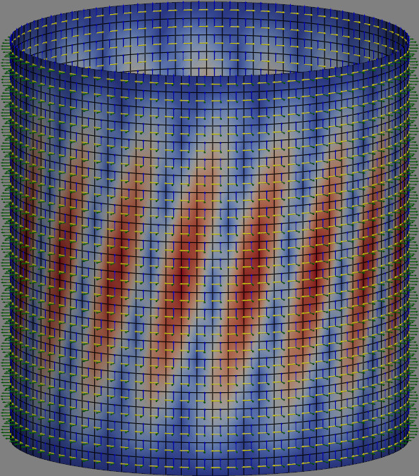
The code used to generate this figure is extracted from one of pyfe3d unit
tests:
import sys
sys.path.append('..')

import time
import numpy as np
from numpy import isclose
from scipy.sparse.linalg import spsolve
from scipy.sparse import coo_matrix

from pyfe3d.shellprop_utils import laminated_plate
from pyfe3d import Quad4, Quad4Data, Quad4Probe, INT, DOUBLE, DOF
from pyfe3d.solver import linear_buckling


def test_linear_buckling_cylinder_Nxy(mode=0, plot_pyvista=False, refinement=1):
    r"""Test case from reference

        Saullo G. P. Castro, Christian Mittelstedt, Francisco A. C. Monteiro, Mariano
        A. Arbelo, Gerhard Ziegmann, Richard Degenhardt. "Linear buckling predictions
        of unstiffened laminated composite cylinders and cones under various loading
        and boundary conditions using semi-analytical models". Composite Structures,
        2014. 10.1016/j.compstruct.2014.07.037

        Cylinders Z11 and Z33 are used given their distinct torsion buckling
        behaviour.

    """
    # NOTE in Fig. 1 of Castro's paper that in their coordinate system a
    # positive angle should be represented also a positive angle here
    # NOTE stacking sequences from Table 4 in Castro et al.
    stacks = {
        # NOTE actual values from reference can be found here https://github.com/saullocastro/compmech/blob/e7e5342bf212743e70da22c94cc0452911099db3/compmech/conecyl/conecylDB.py#L334
        'Z11' : [+60, -60, 0, 0, +68, -68, +52, -52, +37, -37],
        # NOTE actual values from reference can be found here https://github.com/saullocastro/compmech/blob/e7e5342bf212743e70da22c94cc0452911099db3/compmech/conecyl/conecylDB.py#L145
        'Z33' : [0, 0, 19, -19, 37, -37, 45, -45, 51, -51],
    }
    # NOTE the paper is the source of the geometry, the material, the
    #      stacking sequences and the boundary conditions. It does not
    #      tabulate the torsional buckling load: the closest published value
    #      is the intercept of the curves of Fig. 13 (FSDT-BC2, CC2) with the
    #      axis of zero axial load, which is pure torsion. Read off that
    #      figure, those intercepts are about
    #
    #          Z11   -15.4 kNm  and  +16.6 kNm
    #          Z33    -9.3 kNm  and   +9.0 kNm
    #
    #      the two signs differing because the laminates are unsymmetric.
    #      Note that ``Tcr`` below is ``eigval*Nxy*b*R``, which by the sign
    #      convention stated further down is minus the torque T of the paper,
    #      so the magnitudes here are to be compared with the positive
    #      intercepts, +16.6 and +9.0 kNm.
    #
    #      The converged values below are therefore about 16 per cent (Z11)
    #      and 23 per cent (Z33) above the semi-analytical prediction. They
    #      are kept as a regression lock of this element and not as a claim
    #      of agreement with the paper, and the gap is not explained by the
    #      drilling formulation: it is the same for every drilling model and
    #      for both quadrilateral elements, which agree with each other to
    #      about one per cent at this mesh.
    #
    #      The refinement=8 values are mesh converged. For Z11 the critical
    #      mode is a long wave pattern and the sequence over ntheta is
    #
    #          ntheta    40      80     160     320
    #          Tcr   -33163  -22193  -19791  -19214  Nm
    #          waves      8       9      10      10
    #          el/wave  5.0     8.9    16.0    30.4
    #
    #      so the mode is well resolved and the load is settling near
    #      -19.1 kNm, the last step being 2.9 per cent. Torsional buckling is
    #      favourable in this respect: its critical wavelength spans about a
    #      tenth of the circumference. The axial compression of the same
    #      cylinder is not comparable in this way, its critical half
    #      wavelength being of the order of sqrt(R*t) = 17.7 mm, some 89
    #      circumferential waves, so a comparison with Table 6 of the paper
    #      needs a far finer mesh than the ones used here, see
    #      test_quad4_linear_buckling_cylinder_displ.py
    # NOTE values updated in 0.10.0, when the physics-based drilling
    #      stiffness of Allman, Hughes and Brezzi became the default. The
    #      previous values were Z11 -18365.1 and Z33 -10844.0, obtained with
    #      a Quad4 whose drilling penalty coefficient K6ROT*1e-6*A66 had been
    #      lost, leaving an effective coefficient of 1. Restoring that
    #      coefficient alone gives Z11 -19159.9 and Z33 -11091.2, and the new
    #      default gives the values below, only 0.3% and 0.2% away from them.
    #      At this converged mesh the three-way agreement is the useful
    #      check: the restored penalty, the physics-based default and the
    #      Quad4R values -18995.4 and -11032.4 all lie within about 1%,
    #      whereas the lost coefficient put Quad4 3.3% away from Quad4R
    reference_Tcr_value_Castro_refinement_8 = {
        'Z11' : -19214.0,
        'Z33' : -11110.4
    }
    # NOTE values used for CI tests, values derived after running the tests in
    # a local compuer with refinement=8 first and then with refinement=1
    # NOTE values updated in 0.10.0 together with the refinement=8 ones above.
    #      The previous values were Z11 -31583.4 and Z33 -21716.0, and the
    #      restored penalty alone gives Z11 -32074.5 and Z33 -22330.7. This
    #      mesh is far too coarse for the buckling load, roughly 70% above
    #      the converged one, so the coarse-mesh values are a regression lock
    #      and not a measure of accuracy. Running this case with
    #      quad.drilling_model = 1 recovers the penalty values
    reference_Tcr_value_Castro_refinement_1 = {
        'Z11' : -33162.7,
        'Z33' : -23028.4
    }

    for cyl in ['Z11', 'Z33']:
        stack = stacks[cyl]
        if refinement == 1:
            ref_Tcr = reference_Tcr_value_Castro_refinement_1[cyl]
        elif refinement == 8:
            ref_Tcr = reference_Tcr_value_Castro_refinement_8[cyl]
        else:
            raise ValueError('refinement must be 1 or 8')

        data = Quad4Data()
        probe = Quad4Probe()

        L = 0.510 # m
        R = 0.250 # m
        b = 2*np.pi*R # m

        ntheta = 40*refinement # circumferential
        nlength = int(ntheta*L/b)
        if nlength % 2 == 0:
            nlength += 1
        print('ntheta', ntheta)
        print('nlength', nlength)

        # NOTE material proporties from Table 3 in Castro et al.
        # Actual values from reference can be found here https://github.com/saullocastro/compmech/blob/e7e5342bf212743e70da22c94cc0452911099db3/compmech/conecyl/conecylDB.py#L32C34-L32C76
        E11 = 123.55e9
        E22 = 8.708e9
        nu12 = 0.319
        G12 = 5.695e9
        G13 = 5.695e9
        G23 = 3.400e9
        plyt = 0.125e-3
        laminaprop = (E11, E22, nu12, G12, G13, G23)

        # NOTE forcing 5/6 according to Castro et al., beginning of Section 6
        prop = laminated_plate(stack=stack, plyt=plyt, laminaprop=laminaprop,
                               shear_correction='constant')


        nids = 1 + np.arange(nlength*(ntheta+1))
        nids_mesh = nids.reshape(nlength, ntheta+1)
        nids_mesh[:, -1] = nids_mesh[:, 0]
        nids = np.unique(nids_mesh)
        nid_pos = dict(zip(nids, np.arange(len(nids))))

        zlin = np.linspace(0, L, nlength)
        thetatmp = np.linspace(0, 2*np.pi, ntheta+1)
        thetalin = np.linspace(0, 2*np.pi-(thetatmp[-1] - thetatmp[-2]), ntheta)[::-1]
        zmesh, thetamesh = np.meshgrid(zlin, thetalin)
        zmesh = zmesh.T
        thetamesh = thetamesh.T
        xmesh = np.cos(thetamesh)*R
        ymesh = np.sin(thetamesh)*R

        ncoords = np.vstack((xmesh.flatten(), ymesh.flatten(), zmesh.flatten())).T
        ncoords_flatten = ncoords.flatten()
        x = ncoords[:, 0]
        y = ncoords[:, 1]
        z = ncoords[:, 2]

        n1s = nids_mesh[:-1, :-1].flatten()
        n2s = nids_mesh[1:, :-1].flatten()
        n3s = nids_mesh[1:, 1:].flatten()
        n4s = nids_mesh[:-1, 1:].flatten()

        num_elements = len(n1s)
        print('num_elements', num_elements)

        KC0r = np.zeros(data.KC0_SPARSE_SIZE*num_elements, dtype=INT)
        KC0c = np.zeros(data.KC0_SPARSE_SIZE*num_elements, dtype=INT)
        KC0v = np.zeros(data.KC0_SPARSE_SIZE*num_elements, dtype=DOUBLE)
        KGr = np.zeros(data.KG_SPARSE_SIZE*num_elements, dtype=INT)
        KGc = np.zeros(data.KG_SPARSE_SIZE*num_elements, dtype=INT)
        KGv = np.zeros(data.KG_SPARSE_SIZE*num_elements, dtype=DOUBLE)
        N = DOF*nlength*ntheta

        quads = []
        init_k_KC0 = 0
        init_k_KG = 0
        t0 = time.time()
        for n1, n2, n3, n4 in zip(n1s, n2s, n3s, n4s):
            quad = Quad4(probe)
            quad.n1 = n1
            quad.n2 = n2
            quad.n3 = n3
            quad.n4 = n4
            quad.c1 = DOF*nid_pos[n1]
            quad.c2 = DOF*nid_pos[n2]
            quad.c3 = DOF*nid_pos[n3]
            quad.c4 = DOF*nid_pos[n4]
            quad.init_k_KC0 = init_k_KC0
            quad.init_k_KG = init_k_KG
            quad.K6ROT = 100.
            quad.update_rotation_matrix(ncoords_flatten, 0., 0., 1.)
            quad.update_probe_xe(ncoords_flatten)
            quad.update_KC0(KC0r, KC0c, KC0v, prop)
            quads.append(quad)
            init_k_KC0 += data.KC0_SPARSE_SIZE
            init_k_KG += data.KG_SPARSE_SIZE

        print('elements created', time.time()-t0)

        KC0 = coo_matrix((KC0v, (KC0r, KC0c)), shape=(N, N)).tocsc()

        print('sparse KC0 created')

        bk = np.zeros(N, dtype=bool)

        # NOTE cylinders with CC2 boundary condition as decribed in Table 1 of Castro et al.
        bottom_edge = isclose(z, 0)
        bk[0::DOF][bottom_edge] = True
        bk[1::DOF][bottom_edge] = True
        bk[3::DOF][bottom_edge] = True
        bk[4::DOF][bottom_edge] = True

        top_edge = isclose(z, L)
        bk[0::DOF][top_edge] = True
        bk[1::DOF][top_edge] = True
        bk[3::DOF][top_edge] = True
        bk[4::DOF][top_edge] = True

        middle = isclose(z, L/2)
        bk[2::DOF][middle] = True

        bu = ~bk

        # NOTE in Fig. 1 of Castro et al. that a positive torque (T) represents a
        # negative distributed shear force Nxy. This must be consistent with the
        # sign of the stacking sequence angles given that it significantly
        # influences the results for torsion buckling.
        #
        Nxy = -1000/b
        print('Nxy', Nxy)

        for quad in quads:
            quad.update_probe_xe(ncoords_flatten) # NOTE update affects the Quad4Probe class attribute xe
            quad.update_KG_given_stress(0, 0, Nxy, KGr, KGc, KGv)
        KG = coo_matrix((KGv, (KGr, KGc)), shape=(N, N)).tocsc()

        KC0uu = KC0[bu, :][:, bu]
        KGuu = KG[bu, :][:, bu]

        print('sparse KG created')

        num_eig_lb = max(mode+1, 3)

        eigvecs = np.zeros((N, num_eig_lb))

        # NOTE pyfe3d.solver.linear_buckling equilibrates the diagonal,
        #      estimates the Cayley shift and verifies that no lower load
        #      multiplier was missed, which a hardcoded shift does not
        eigvals, eigvecsu = linear_buckling(KC0uu, KGuu, num_eigvalues=num_eig_lb, tol=1e-9)

        eigvecs[bu] = eigvecsu
        print('eigvals', eigvals)

        print('linear buckling analysis OK')
        Tcr = eigvals[0]*Nxy*b*R
        print('Tcr =', Tcr)

        if plot_pyvista:
            import pyvista as pv

            contour_colorscale = 'coolwarm'
            background = 'gray'

            vector = eigvecs[:, mode]

            contour_label = 'Radial displacement'
            contour_vec = np.sqrt(vector[0::DOF]**2 + vector[1::DOF]**2)

            displ_vec = np.zeros_like(ncoords)
            displ_vec[:, 0] = vector[0::DOF]*10
            displ_vec[:, 1] = vector[1::DOF]*10
            displ_vec[:, 2] = vector[2::DOF]*10
            intensitymode = 'vertex'

            plotter = pv.Plotter(off_screen=False)
            faces_quad = []
            for q in quads:
                faces_quad.append([4, nid_pos[q.n1], nid_pos[q.n2], nid_pos[q.n3], nid_pos[q.n4]])
            faces_quad = np.array(faces_quad)
            quad_plot = pv.PolyData(ncoords, faces_quad)
            if contour_vec is not None:
                quad_plot[contour_label] = contour_vec
                plotter.add_mesh(quad_plot, scalars=contour_label,
                        cmap=contour_colorscale, edge_color='black', show_edges=True,
                        line_width=1.)
            else:
                plotter.add_mesh(quad_plot, edge_color='black', show_edges=True,
                        line_width=1.)
            displ_vec = None
            if displ_vec is not None:
                quad_plot = pv.PolyData(ncoords + displ_vec, faces_quad)
                plotter.add_mesh(quad_plot, edge_color='red', show_edges=True,
                        line_width=1., opacity=0.5)
            #NOTE plotting coordinate system
            xaxis = pv.Arrow(start=(0, 0, 0), direction=(1, 0, 0), scale=R/3)
            plotter.add_mesh(xaxis, color='blue')
            yaxis = pv.Arrow(start=(0, 0, 0), direction=(0, 1, 0), scale=R/3)
            plotter.add_mesh(yaxis, color='yellow')
            zaxis = pv.Arrow(start=(0, 0, 0), direction=(0, 0, 1), scale=R/3)
            plotter.add_mesh(zaxis, color='green')

            for q in quads:
                pos1 = nid_pos[q.n1]
                pos2 = nid_pos[q.n2]
                pos3 = nid_pos[q.n3]
                pos4 = nid_pos[q.n4]
                centroid = (ncoords[pos1] + ncoords[pos2] + ncoords[pos3] + ncoords[pos4])/4
                ze = np.array([0., 0., 1.])
                zg = np.array([[q.r11, q.r12, q.r13],
                               [q.r21, q.r22, q.r23],
                               [q.r31, q.r32, q.r33]]) @ ze
                normal = pv.Arrow(start=centroid, direction=zg, scale=R/20)
                plotter.add_mesh(normal, color='green')

                xe = np.array([1., 0., 0.])
                xg = np.array([[q.r11, q.r12, q.r13],
                               [q.r21, q.r22, q.r23],
                               [q.r31, q.r32, q.r33]]) @ xe
                x_axis = pv.Arrow(start=centroid, direction=xg, scale=R/20)
                plotter.add_mesh(x_axis, color='blue')

                ye = np.array([0., 1., 0.])
                yg = np.array([[q.r11, q.r12, q.r13],
                               [q.r21, q.r22, q.r23],
                               [q.r31, q.r32, q.r33]]) @ ye
                y_axis = pv.Arrow(start=centroid, direction=yg, scale=R/20)
                plotter.add_mesh(y_axis, color='yellow')

            plotter.set_background(background)
            plotter.parallel_projection = True
            plotter.show()

        assert np.isclose(Tcr, ref_Tcr, rtol=1e-3)


if __name__ == '__main__':
    test_linear_buckling_cylinder_Nxy(mode=0, plot_pyvista=False, refinement=8)