Quad4 - Quadrilateral element with mixed integration (`pyfe3d.quad4`)#

The Quad4 is the recommended quadrilateral plane stress finite element.

Another option is the pyfe3d.Quad4R with full reduced integration, more efficient, but with an hourglass control that creates artificial stiffness to compensate the reduced integration.

The Quad4 element has 6 degrees-of-freedom (DOF): \(u\), \(v\), \(w\), \(r_x\), \(r_y\), \(r_z\). All DOF are interpolated bi-linearly between the nodes, such that any of the DOF gradients can be constant over the element when the element is rectangular.

The stiffness for the degrees of freedom \(w\), \(r_x\) and \(r_y\) is based on the paper below, where \(r_x = \theta_1\) and \(r_y = \theta_2\):

Hughes T.J.R., Taylor R.L., Kanoknukulchai W. “A simple and efficient finite element for plate bending”. International Journal of Numerical Methods in Engineering, Volume 11, 1977. https://doi.org/10.1002/nme.1620111005

Hughes et al. (1977) proposed the following integration scheme:

For thin plates, when \(h/\ell < 1\), where \(\ell\) is the element characteristic length, here calculated as the square root of the element area \(\ell = \sqrt{\text{area}}\)

– two-by-two quadrature for the bending energy terms

– one-point quadrature for the transverse shear energy terms

For thick plates, when \(h/\ell >= 1\)

– two-by-two quadrature for the bending energy terms

– two-by-two quadrature for the transverse shear terms with gradients

– one-point quadrature for the transverse shear terms without gradients

The membrane stiffness terms, which are not specified in the paper of Hughes et al. (1977), are integrated with a three-by-three quadrature when the default drilling model is active and with a two-by-two quadrature otherwise, for the reason explained under the drilling stiffness below. The bending term always uses two-by-two, so that the drilling model does not change the bending response of the element.

The transverse shear stiffnesses \(A_{44}\), \(A_{45}\) and \(A_{55}\) are read from the pyfe3d.shellprop.ShellProp object with the shear correction already applied, see pyfe3d.shellprop.ShellProp.calc_transverse_shear_stiffness(), and no shear correction factor is applied by the element. When a material direction is defined, they are brought to the element coordinate system with pyfe3d.shellprop.ShellProp.calc_Ats_element(), which re-evaluates the equilibrium-based stiffness of Rohwer (1988) with the plies rotated to the element coordinate system, such that the assumed cylindrical bending states are posed along the element axes.

Drilling stiffness#

The FSDT kinematics contains no strain measure associated with \(r_z\), so the rows and columns of the drilling degree-of-freedom would be empty and a mesh of coplanar elements would give a singular global stiffness matrix. Two models are available, selected with the drilling_model attribute.

Physics-based, the default (drilling_model = 0). The in-plane displacement field is enriched so that the drilling rotations produce membrane strain energy, following Allman, and the independently interpolated \(r_z\) is tied to the rotation of the membrane field by the regularised functional of Hughes and Brezzi. The combination for the quadrilateral is the one of Ibrahimbegovic, Taylor and Wilson:

Allman, D. J., 1984, “A compatible triangular element including vertex rotations for plane elasticity analysis,” Computers & Structures, 19(1-2), pp. 1-8. https://doi.org/10.1016/0045-7949(84)90197-4

Hughes, T. J. R., and Brezzi, F., 1989, “On drilling degrees of freedom,” Computer Methods in Applied Mechanics and Engineering, 72(1), pp. 105-121. https://doi.org/10.1016/0045-7825(89)90124-2

Ibrahimbegovic, A., Taylor, R. L., and Wilson, E. L., 1990, “A robust quadrilateral membrane finite element with drilling degrees of freedom,” International Journal for Numerical Methods in Engineering, 30(3), pp. 445-457. https://doi.org/10.1002/nme.1620300305

Each edge \(k\), joining nodes \(i\) and \(j\) and of length \(\ell_k\), carries a quadratic normal displacement whose end slopes are identified with the vertex drilling rotations, giving the amplitude

\[a_k = \frac{\ell_k}{8}\left({r_z}_i - {r_z}_j\right)\]

so that the enrichment is not a new degree-of-freedom but the difference of the two drilling rotations already present at the ends of the edge. The in-plane field becomes

\[\begin{split}\left\{\begin{matrix} u \\ v \end{matrix}\right\} = \sum_i S_i \left\{\begin{matrix} u_i \\ v_i \end{matrix}\right\} + \sum_k N_k \frac{\ell_k}{8}\left({r_z}_i - {r_z}_j\right) \pmb{n}_k\end{split}\]

with \(\pmb{n}_k\) the unit normal of edge \(k\) and \(N_k\) the hierarchical bubble of that edge, equal to unity at its mid-point and zero at every corner, which for the quadrilateral are the mid-side functions of the eight-node serendipity element. In row form the enrichment populates the drilling columns of the membrane operator, giving \(\pmb{\tilde B}_m\), whereas the curvature and transverse shear operators are untouched, because the edge modes act only on the in-plane translations. The drilling residual becomes

\[\pmb{\tilde B}_{r_z} = \pmb{S}^{r_z} + \frac{1}{2}\pmb{\tilde S}^u_{,y} - \frac{1}{2}\pmb{\tilde S}^v_{,x}\]

and the contribution to the element stiffness matrix is

\[\pmb{K}_{r_z} = \gamma_{r_z} \iint_{\xi\eta} \pmb{\tilde B}_{r_z}^\top \pmb{\tilde B}_{r_z} \det \pmb{J} d\xi d\eta \qquad \text{with} \qquad \gamma_{r_z} = A_{66}\]

The value \(\gamma_{r_z} = A_{66}\) is a modulus and not a user parameter. Hughes and Brezzi identify the shear modulus \(G\) as the natural regularisation parameter of the isotropic problem, and the thickness integration turns \(G\) into \(hG = A_{66}\), which generalises to the \(A_{66}\) of the laminate extensional stiffness matrix. The gamma_rz attribute allows a different value to be used, which is only of interest for the sensitivity study that the literature recommends.

Allman’s enrichment on its own is rank-deficient by one, because the state \(u_i = v_i = 0\) with \({r_z}_i = \omega_0\) makes every amplitude \(a_k\) vanish and therefore produces no membrane strain, although it is not a rigid-body motion. The term above gives that state the energy \(\frac{1}{2}\gamma_{r_z} A_e \omega_0^2\), with \(A_e\) the element area, and restores the rank, which is why the two ingredients are used together.

Two quadrature choices matter and both follow Ibrahimbegovic et al. (1990). The membrane term is integrated with three points per direction: the edge modes make \(\pmb{\tilde B}_m\) vary linearly, and with two points the alternating pattern of the drilling rotations produces no membrane strain at any of the four points, leaving a zero-energy mode that no value of \(\gamma_{r_z}\) can remove. The constraint term \(\pmb{K}_{r_z}\) is integrated with a single point at the centroid, which is what makes the element insensitive to \(\gamma_{r_z}\): a fully integrated constraint over-constrains \(r_z = \theta_z\) and locks the membrane response as \(\gamma_{r_z}\) grows, whereas with one point the response reaches an asymptote. One point also gives the constraint rank one per element, exactly what is needed to remove the uniform drilling mode.

Unlike the penalty below, the added term is consistent rather than artificial. Stationarity with respect to \(r_z\) gives \(\gamma_{r_z}(r_z - \theta_z) = 0\) pointwise, so the exact solution satisfies \(r_z = \theta_z\) and the term contributes no energy, for any positive \(\gamma_{r_z}\). The nodal moments about the shell normal recovered in the internal force vector are therefore physical, and in-plane moments can be transmitted between shells and beams through the shared drilling degree-of-freedom. Note also that when \(\pmb{B} \neq \pmb{0}\), for an offset reference surface or an unsymmetric laminate, the enriched membrane operator couples \(r_z\) to the curvatures, which is physically correct.

Fictitious penalty (drilling_model = 1), the default before version 0.10.0, following the approach adopted in MSC Nastran and Autodesk Nastran through their K6ROT parameter. It provides a small artificial stiffness whose only purpose is to remove the singularity, so the forces associated with it are spurious and any moment recovered about the shell normal is meaningless. The penalty energy is defined per element as:

\[U_{drill} = \frac{1}{2} K6ROT \cdot 10^{-6} \cdot \int_A A_{66} (r_z - \theta_z)^2 dA\]

where \(10^{-6}\) is a scaling factor suggested by MSC Nastran’s approach (CQUAD4) to make the artificial drilling stiffness sufficiently small. AUTODESK NASTRAN’s quick reference guide recommends \(K6ROT = 100\) for static analysis. For modal solutions, \(K6ROT = 10^4\) is suggested. MSC NASTRAN’s quick reference guide states that \(K6ROT > 100\) should not be used, thus contradicting AUTODESK NASTRAN. The rotation \(r_z\) represents the drilling degree-of-freedom in element’s coordinates, whereas \(\theta_z\) the in-plane rotation strain, defined as:

\[\theta_z = \frac{1}{2}\left(\frac{\partial v}{\partial x} - \frac{\partial u}{\partial y}\right)\]

The first variation of U_{drill} then becomes:

\[\delta U_{drill} = K6ROT \cdot 10^{-6} \cdot \int_A A_{66} (r_z - \theta_z)(\delta r_z - \delta \theta_z) dA\]

which can be expressed in terms of the shape functions and element degrees-of-freedom (\(u_e\)) as: \(r_z = S^{r_z} u_e\), \(u = S^u u_e\) and \(v = S_v u_e\) as:

\[\delta U_{drill} = K6ROT \cdot 10^{-6} \cdot u_e^\top \int_A A_{66} (S^{r_z \top} + 1/2 S^{u \top}_{,y} - 1/2 S^{v \top}_{,x})(\delta S^{r_z} + 1/2 \delta S^u_{,y} - 1/2 S^v_{,x}) dA u_e\]

or simply as:

\[\delta U_{drill} = K6ROT \cdot 10^{-6} \cdot A_{66} u_e^\top \int_A B_{drill}^\top B_{drill} dA u_e\]

with:

\[B_{drill} = S^{r_z} + 1/2 S^u_{,y} - 1/2 S^v_{,x}\]

which is the same operator as \(\pmb{\tilde B}_{r_z}\) above, evaluated on the unenriched field. Being built from that operator and not from an addition on the diagonal terms is what keeps the penalty from stiffening a rigid rotation of the element about its normal, so both models represent all rigid-body motions and all constant-strain states exactly. \(A_{66}\) is assumed constant over the element. This term is integrated with the two-by-two quadrature. The approach herein presented is very similar to the one presented in Eq. 2.20 of:

Adam, F. M., Mohamed, A. E., and Hassaballa, A. E., 2013, u201cDegenerated Four Nodes Shell Element with Drilling Degree of Freedom,u201d IOSR J. Eng., 3(8), pp. 10u201320.

Choosing between them. The physics-based model is the default because it is the one that is correct when the drilling moment is part of the load path, when shells are connected to beams or stiffeners that must transmit in-plane moments, or when the mesh is too coarse for the unenriched membrane response to be trusted. It is markedly more accurate in in-plane bending: on Cook’s skew membrane with a two-by-two mesh it gives 20.8 against the reference 23.9, where the penalty gives 11.8. The penalty remains available for reproducing results obtained before 0.10.0, and it is cheaper, since it leaves the membrane term on the two-by-two quadrature.

class pyfe3d.quad4.Quad4#

Nodal connectivity for the plate element similar to Nastran’s CQUAD4:

 ^ y
 |
4 ________ 3
 |       |
 |       |   --> x
 |       |
 |_______|
1         2

The element coordinate system is determined identically what is explained in Nastran’s quick reference guide for the CQUAD4 element, as illustrated below.

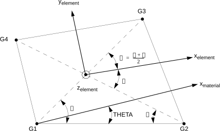
Attributes:

eid,int: Element identification number.
pid,int: Property identification number.
area,double: Element area.
drilling_model,int: Selects how the drilling degree-of-freedom \(r_z\) is given stiffness, see the module documentation. The default 0 is the physics-based stiffness, combining the in-plane enrichment of Allman (1984) with the regularisation of Hughes and Brezzi (1989), in the form given for the quadrilateral by Ibrahimbegovic et al. (1990). With it the drilling rotation is a kinematic variable that carries strain energy, the recovered nodal moments about the shell normal are physical, and no user parameter is involved. Any other value selects the fictitious penalty of MSC Nastran and Autodesk Nastran, which was the default up to version 0.9.0 and is controlled by K6ROT. Setting elem.drilling_model = 1 before calling update_KC0() is the way to reproduce results obtained before 0.10.0.

Note

The attribute must be set before the element matrices are updated, and the same value must be passed to Quad4Probe.update_BL() when strains are recovered from the probe.
K6ROT,double: Dimensionless multiplier for the fictitious drilling stiffness, only read when drilling_model is not 0. It has no effect under the default physics-based model, which takes its regularisation parameter from the laminate stiffness instead, see gamma_rz. AUTODESK NASTRAN’s quick reference guide recommends K6ROT = 100. for static analysis. For modal solutions, K6ROT=1.e4 is suggested. MSC NASTRAN’s quick reference guide states that K6ROT > 100. should not be used, but this is contradicting AUTODESK NASTRAN.
gamma_rz,double: Regularisation parameter \(\gamma_{r_z}\) of the physics-based drilling stiffness, only read when drilling_model is 0. The default is a negative value, which means that \(A_{66}\) of the laminate extensional stiffness matrix is used, the value identified by Hughes and Brezzi (1989). This is a modulus and not a parameter that needs tuning: the element response has a broad plateau of insensitivity around it, and the attribute is exposed for the sensitivity study that the literature recommends rather than for normal use. Very large values over-constrain \(r_z = \theta_z\), and a zero value leaves the Allman enrichment rank-deficient by one.
r11, r12, r13, r21, r22, r23, r31, r32, r33double: Rotation matrix from local to global coordinates.
m11, m12, m21, m22double: Rotation matrix only for the constitutive relations. Used when a material direction is used instead of the element local coordinates.
c1, c2, c3, c4int: Position of each node in the global stiffness matrix.
n1, n2, n3, n4int: Node identification number.
init_k_KC0, init_k_KCNL, init_k_KG, init_k_Mint: Position in the arrays storing the sparse data for the structural matrices.
init_k_KA_beta, init_k_KA_gamma, init_k_CAint: Position in the arrays storing the sparse data for the aerodynamic matrices based on the Piston theory.
probe,Quad4Probe object: Pointer to the probe.

Methods

`update_CA`(self, long[, long[, double[)	Update sparse vectors for piston-theory aerodynamic damping matrix \(CA\)
`update_KA_beta`(self, long[, long[, double[)	Update sparse vectors for piston-theory aerodynamic matrix \(KA_{\beta}\)
`update_KA_gamma`(self, long[, long[, double[)	Update sparse vectors for piston-theory aerodynamic matrix \(KA_{\gamma}\)
`update_KC0`(self, long[, long[, double[, ...)	Update sparse vectors for linear constitutive stiffness matrix KC0
`update_KCNL`(self, long[, long[, double[, ...)	Update sparse vectors for the nonlinear constitutive stiffness matrix KCNL
`update_KG`(self, long[, long[, double[, ...)	Update sparse vectors for geometric stiffness matrix KG
`update_KG_given_stress`(self, double Nxx, ...)	Update sparse vectors for geometric stiffness matrix KG
`update_M`(self, long[, long[, double[, ...)	Update sparse vectors for mass matrix M
`update_area`(self)	Update element area
`update_fint`(self, double[, ShellProp prop, ...)	Update the internal force vector
`update_probe_finte`(self, ShellProp prop, ...)	Update the internal force vector of the probe
`update_probe_ue`(self, double[)	Update the local displacement vector of the probe of the element
`update_probe_xe`(self, double[)	Update the 3D coordinates of the probe of the element
`update_rotation_matrix`(self, double[, ...)	Update the rotation matrix of the element

K6ROT#: K6ROT: ‘double’

area#: area: ‘double’

c1#: c1: ‘int’

c2#: c2: ‘int’

c3#: c3: ‘int’

c4#: c4: ‘int’

drilling_model#: drilling_model: ‘int’

eid#: eid: ‘int’

gamma_rz#: gamma_rz: ‘double’

init_k_CA#: init_k_CA: ‘int’

init_k_KA_beta#: init_k_KA_beta: ‘int’

init_k_KA_gamma#: init_k_KA_gamma: ‘int’

init_k_KC0#: init_k_KC0: ‘int’

init_k_KCNL#: init_k_KCNL: ‘int’

init_k_KG#: init_k_KG: ‘int’

init_k_M#: init_k_M: ‘int’

m11#: m11: ‘double’

m12#: m12: ‘double’

m21#: m21: ‘double’

m22#: m22: ‘double’

n1#: n1: ‘int’

n2#: n2: ‘int’

n3#: n3: ‘int’

n4#: n4: ‘int’

pid#: pid: ‘int’

probe#: probe: pyfe3d.quad4.Quad4Probe

r11#: r11: ‘double’

r12#: r12: ‘double’

r13#: r13: ‘double’

r21#: r21: ‘double’

r22#: r22: ‘double’

r23#: r23: ‘double’

r31#: r31: ‘double’

r32#: r32: ‘double’

r33#: r33: ‘double’

update_CA(self, long[: :1] CAr, long[: :1] CAc, double[: :1] CAv) → void#

Update sparse vectors for piston-theory aerodynamic damping matrix \(CA\)

Parameters:

CArnp.array: Array to store row positions of sparse values
CAcnp.array: Array to store column positions of sparse values
CAvnp.array: Array to store sparse values

update_KA_beta(self, long[: :1] KA_betar, long[: :1] KA_betac, double[: :1] KA_betav) → void#

Update sparse vectors for piston-theory aerodynamic matrix \(KA_{\beta}\)

Parameters:

KA_betarnp.array: Array to store row positions of sparse values
KA_betacnp.array: Array to store column positions of sparse values
KA_betavnp.array: Array to store sparse values

update_KA_gamma(self, long[: :1] KA_gammar, long[: :1] KA_gammac, double[: :1] KA_gammav) → void#

Update sparse vectors for piston-theory aerodynamic matrix \(KA_{\gamma}\)

Parameters:

KA_gammarnp.array: Array to store row positions of sparse values
KA_gammacnp.array: Array to store column positions of sparse values
KA_gammavnp.array: Array to store sparse values

update_KC0(self, long[: :1] KC0r, long[: :1] KC0c, double[: :1] KC0v, ShellProp prop, int update_KC0v_only=0) → void#

Update sparse vectors for linear constitutive stiffness matrix KC0

Parameters:

KC0rnp.array: Array to store row positions of sparse values
KC0cnp.array: Array to store column positions of sparse values
KC0vnp.array: Array to store sparse values
propShellProp object: Shell property object from where the stiffness and mass attributes are read from.
update_KC0v_onlyint: The default 0 means that the row and column indices KC0r and KC0c should also be updated. Any other value will only update the stiffness matrix values KC0v.

update_KCNL(self, long[: :1] KCNLr, long[: :1] KCNLc, double[: :1] KCNLv, ShellProp prop, int update_KCNLv_only=0) → void#

Update sparse vectors for the nonlinear constitutive stiffness matrix KCNL

Assuming that KCNL = KC0L + KCL0 + KCLL + KGNL, built from the von Karman membrane strains

\[\epsilon_{xx} = u_{,x} + \frac{1}{2} w_{,x}^2, \quad \epsilon_{yy} = v_{,y} + \frac{1}{2} w_{,y}^2, \quad \gamma_{xy} = u_{,y} + v_{,x} + w_{,x} w_{,y}\]

whose nonlinear part is \(\{\epsilon_{NL}\} = \frac{1}{2} [B_{mL}] \{u_e\}\), with \([B_{mL}]\) its variation. With \([B_m]\) and \([B_b]\) the linear membrane and bending strain-displacement matrices, \([G]\) the gradient of \(w\), and \([A]\), \([B]\) the laminate matrices:

KC0L = \([B_m]^T [A] [B_{mL}] + [B_b]^T [B] [B_{mL}]\)
KCL0 = KC0L`^T`
KCLL = \([B_{mL}]^T [A] [B_{mL}]\)
KGNL = \([G]^T [N_{NL}] [G]\), with \(\{N_{NL}\} = [A] \{\epsilon_{NL}\}\)

The first three groups are the constitutive terms coupling the linear and the nonlinear parts of the membrane strain. KGNL is geometric, carrying the stress of the nonlinear membrane strain. It is collected here so that update_KG() stays homogeneous of degree one in the displacements, which is what a linear buckling analysis needs. With it here,

\[K_T = K_{C0} + K_{CNL}(u) + K_G(u)\]

is the exact Jacobian of the internal forces of update_fint() with nonlinear=1, and a Newton-Raphson iteration built on them converges quadratically. The quadrature of update_KG() is used.

Before this function is called, the probe Quad4Probe attribute of the Quad4 object must be updated using update_probe_ue() with the current displacements; and update_probe_xe() with the node coordinates.

Parameters:

KCNLrnp.array: Array to store row positions of sparse values
KCNLcnp.array: Array to store column positions of sparse values
KCNLvnp.array: Array to store sparse values
propShellProp object: Shell property object from where the stiffness and mass attributes are read from.
update_KCNLv_onlyint: The default 0 means that the row and column indices KCNLr and KCNLc should also be updated. Any other value will only update the stiffness matrix values KCNLv.

update_KG(self, long[: :1] KGr, long[: :1] KGc, double[: :1] KGv, ShellProp prop) → void#

Update sparse vectors for geometric stiffness matrix KG

Two-point Gauss-Legendre quadrature is used, which showed more accuracy for linear buckling load predictions.

Before this function is called, the probe Quad4Probe attribute of the Quad4 object must be updated using update_probe_ue() with the correct pre-buckling (fundamental state) displacements; and update_probe_xe() with the node coordinates.

Parameters:

KGrnp.array: Array to store row positions of sparse values
KGcnp.array: Array to store column positions of sparse values
KGvnp.array: Array to store sparse values
propShellProp object: Shell property object from where the stiffness and mass attributes are read from.

update_KG_given_stress(self, double Nxx, double Nyy, double Nxy, long[: :1] KGr, long[: :1] KGc, double[: :1] KGv) → void#

Update sparse vectors for geometric stiffness matrix KG

Note

A constant stress state is assumed within the element, according to the given values of \(N_{xx}, N_{yy}, N_{xy}\).

Two-point Gauss-Legendre quadrature is used, which showed more accuracy for linear buckling load predictions.

Before this function is called, the probe Quad4Probe attribute of the Quad4 object must be updated using update_probe_xe() with the node coordinates.

Parameters:

KGrnp.array: Array to store row positions of sparse values
KGcnp.array: Array to store column positions of sparse values
KGvnp.array: Array to store sparse values

update_M(self, long[: :1] Mr, long[: :1] Mc, double[: :1] Mv, ShellProp prop, int mtype=0) → void#

Update sparse vectors for mass matrix M

Different integration schemes are available by means of the mtype parameter.

Parameters:

Mrnp.array: Array to store row positions of sparse values
Mcnp.array: Array to store column positions of sparse values
Mvnp.array: Array to store sparse values
mtypeint, optional: 0 for consistent mass matrix using method from Brockman 1987 1 for reduced integration mass matrix using method from Brockman 1987 2 for lumped mass matrix using method from Brockman 1987

update_area(self) → void#: Update element area

update_fint(self, double[: :1] fint, ShellProp prop, int nonlinear=0) → void#

Update the internal force vector

Parameters:

fintnp.array: Array that is updated in place with the internal forces. The internal forces stored in fint are calculated in global coordinates. Method update_probe_finte() is called to update the parameter finte of the Quad4Probe with the internal forces in local coordinates.
propShellProp object: Shell property object from where the stiffness and mass attributes are read from.
nonlinearint: The default 0 gives the linear internal forces, KC0*u. Any other value adds the geometrically nonlinear terms of the von Karman strains, for which the exact Jacobian of the internal forces is KC0 + KCNL + KG, see update_KCNL().

update_probe_finte(self, ShellProp prop, int nonlinear=0) → void#

Update the internal force vector of the probe

The attribute finte of the object Quad4Probe is updated, which corresponds to the internal forces in local coordinates. While using this function, mind that the probe can be shared amongst more than one finite element, depending how you defined them, meaning that the probe will always safe the values from the last udpate.

Note

The finte attribute of object Quad4Probe is updated, accessible using .probe.finte.

Parameters:

propShellProp object: Shell property object from where the stiffness and mass attributes are read from.
nonlinearint: The default 0 gives the linear internal forces, KC0*u. Any other value adds the geometrically nonlinear terms of the von Karman strains, for which the exact Jacobian of the internal forces is KC0 + KCNL + KG, see update_KCNL().

update_probe_ue(self, double[: :1] u) → void#

Update the local displacement vector of the probe of the element

Note

The ue attribute of object Quad4Probe is updated, accessible using .probe.ue.

Parameters:

uarray-like: Array with global displacements, for a total of \(M\) nodes in the model, this array will be arranged as: \(u_1, v_1, w_1, {r_x}_1, {r_y}_1, {r_z}_1, u_2, v_2, w_2, {r_x}_2, {r_y}_2, {r_z}_2, ..., u_M, v_M, w_M, {r_x}_M, {r_y}_M, {r_z}_M\).

update_probe_xe(self, double[: :1] x) → void#

Update the 3D coordinates of the probe of the element

Note

The xe attribute of object Quad4Probe is updated, accessible using .probe.xe.

Parameters:

xarray-like: Array with global nodal coordinates, for a total of \(M\) nodes in the model, this array will be arranged as: \(x_1, y_1, z_1, x_2, y_2, z_2, ..., x_M, y_M, z_M\).

update_rotation_matrix(self, double[: :1] x, double xmati=0., double xmatj=0., double xmatk=0.) → void#

Update the rotation matrix of the element

Attributes r11,r12,r13,r21,r22,r23,r31,r32,r33 are updated, corresponding to the rotation matrix from local to global coordinates.

The element coordinate system is determined, identifying the \(ijk\) components of each axis: \({x_e}_i, {x_e}_j, {x_e}_k\); \({y_e}_i, {y_e}_j, {y_e}_k\); \({z_e}_i, {z_e}_j, {z_e}_k\).

The rotation matrix terms are calculated after solving 9 equations.

Parameters:

xarray-like: Array with global nodal coordinates, for a total of \(M\) nodes in the model, this array will be arranged as: \(x_1, y_1, z_1, x_2, y_2, z_2, ..., x_M, y_M, z_M\).
xmati, xmatj, xmatk: array-like: Vector in global coordinates representing the material direction. This vector is projected onto the plate element, thus becoming the material direction. The \(ABD\) matrix defining the constitutive behavior of the element is rotated from the material direction to the element \(x\) axis while calculating the stiffness matrices.

class pyfe3d.quad4.Quad4Data#

Used to allocate memory for the sparse matrices.

Attributes:

KC0_SPARSE_SIZE,int: KC0_SPARSE_SIZE = 576
KCNL_SPARSE_SIZE,int: KCNL_SPARSE_SIZE = 576
KG_SPARSE_SIZE,int: KG_SPARSE_SIZE = 144
M_SPARSE_SIZE,int: M_SPARSE_SIZE = 480
KA_BETA_SPARSE_SIZE,int: KA_BETA_SPARSE_SIZE = 144
KA_GAMMA_SPARSE_SIZE,int: KA_GAMMA_SPARSE_SIZE = 144
CA_SPARSE_SIZE,int: CA_SPARSE_SIZE = 144

CA_SPARSE_SIZE#: CA_SPARSE_SIZE: ‘int’

KA_BETA_SPARSE_SIZE#: KA_BETA_SPARSE_SIZE: ‘int’

KA_GAMMA_SPARSE_SIZE#: KA_GAMMA_SPARSE_SIZE: ‘int’

KC0_SPARSE_SIZE#: KC0_SPARSE_SIZE: ‘int’

KCNL_SPARSE_SIZE#: KCNL_SPARSE_SIZE: ‘int’

KG_SPARSE_SIZE#: KG_SPARSE_SIZE: ‘int’

M_SPARSE_SIZE#: M_SPARSE_SIZE: ‘int’

class pyfe3d.quad4.Quad4Probe#

Probe used for local coordinates, local displacements, local stiffness, local stresses etc…

The idea behind using a probe is to avoid allocating larger memory buffers per finite element. The memory buffers are allocated per probe, and one probe can be shared amongst many finite elements, with the information being updated and retrieved on demand.

Note

The probe can be shared amongst more than one finite element, depending on how you defined them. Mind that the probe will always safe the values from the last udpate.

Attributes:

xe,array-like: Array of size NUM_NODES*DOF//2=12 containing the nodal coordinates in the element coordinate system, in the following order \({x_e}_1, {y_e}_1, {z_e}_1, `{x_e}_2, {y_e}_2, {z_e}_2\), \({x_e}_3, {y_e}_3, {z_e}_3\), \({x_e}_4, {y_e}_4, {z_e}_4\).
ue,array-like: Array of size NUM_NODES*DOF=24 containing the element displacements in the following order \({u_e}_1, {v_e}_1, {w_e}_1, {{r_x}_e}_1, {{r_y}_e}_1, {{r_z}_e}_1\), \({u_e}_2, {v_e}_2, {w_e}_2, {{r_x}_e}_2, {{r_y}_e}_2, {{r_z}_e}_2\), \({u_e}_3, {v_e}_3, {w_e}_3, {{r_x}_e}_3, {{r_y}_e}_3, {{r_z}_e}_3\), \({u_e}_4, {v_e}_4, {w_e}_4, {{r_x}_e}_4, {{r_y}_e}_4, {{r_z}_e}_4\).
finte,array-like: Array of size NUM_NODES*DOF=24 containing the element internal forces corresponding to the degrees-of-freedom described by ue.
KC0ve,array-like: Local stiffness matrix stored as a 1D array of size (NUM_NODES*DOF)**2.
BLexx, BLeyy, BLgxyarray-like: Arrays of size NUM_NODES*DOF=24 containing the in-plane strain interpolation functions evaluated at a given natural coordinate point \(\xi\), \(\eta\).
BLkxx, BLkyy, BLkxyarray-like: Arrays of size NUM_NODES*DOF=24 containing the bending strain interpolation functions evaluated at a given natural coordinate point \(\xi\), \(\eta\).
BLgyz_grad, BLgyz_rot, BLgxz_grad, BLgxz_rotarray-like: Arrays of size NUM_NODES*DOF=24 containing the transverse shear strain interpolation functions evaluated at a given natural coordinate point \(\xi\), \(\eta\).
BLdrillingarray-like: BLdrilling: ‘double[::1]’
Gwx, Gwyarray-like: Arrays of size NUM_NODES*DOF=24 with the rows giving \(w_{,x}\) and \(w_{,y}\), at the last evaluated integration point.
KCNLvearray-like: KCNLve: ‘double[::1]’

Methods

update_BL(self, double xi, double eta, ...)

Update all components of the interpolation matrix \(\pmb{B_L}\) at a given natural coordinate point \(\xi\), \(\eta\).

BLdrilling#: BLdrilling: ‘double[::1]’

BLexx#: BLexx: ‘double[::1]’

BLeyy#: BLeyy: ‘double[::1]’

BLgxy#: BLgxy: ‘double[::1]’

BLgxz_grad#: BLgxz_grad: ‘double[::1]’

BLgxz_rot#: BLgxz_rot: ‘double[::1]’

BLgyz_grad#: BLgyz_grad: ‘double[::1]’

BLgyz_rot#: BLgyz_rot: ‘double[::1]’

BLkxx#: BLkxx: ‘double[::1]’

BLkxy#: BLkxy: ‘double[::1]’

BLkyy#: BLkyy: ‘double[::1]’

Gwx#: Gwx: ‘double[::1]’

Gwy#: Gwy: ‘double[::1]’

KC0ve#: KC0ve: ‘double[::1]’

KCNLve#: KCNLve: ‘double[::1]’

finte#: finte: ‘double[::1]’

ue#: ue: ‘double[::1]’

update_BL(self, double xi, double eta, int drilling_model=0) → void#

Update all components of the interpolation matrix \(\pmb{B_L}\) at a given natural coordinate point \(\xi\), \(\eta\).

Parameters:

xi, etadouble: Natural coordinates of the evaluation point.
drilling_modelint: Must match the drilling_model attribute of the finite element that the probe is being used with, such that the recovered strains correspond to the displacement field that produced the stiffness matrix. The default 0 includes the Allman drilling enrichment in the membrane rows and in BLdrilling; any other value gives the unenriched rows used by the K6ROT penalty model.

xe#: xe: ‘double[::1]’

Quad4 - Quadrilateral element with mixed integration (pyfe3d.quad4)#

Drilling stiffness#

Quad4 - Quadrilateral element with mixed integration (`pyfe3d.quad4`)#