Tria3R - Triangular element with reduced integration (`pyfe3d.tria3r`)#

Triangular element with reduced integration, where a single point at the centroid (\(N1=N2=N3=1/3\)) and weight \(weight=1\) is evaluated, preventing shear locking. The drilling stiffness is evaluated with full integration.

The transverse shear stiffnesses \(E_{44}\), \(E_{45}\) and \(E_{55}\) are stabilised using the Stenberg’s method described in:

Bischoff, M., & Bletzinger, K.-U. (2004). Improving stability and accuracy of Reissner–Mindlin plate finite elements via algebraic subgrid scale stabilization. Computer Methods in Applied Mechanics and Engineering, 193(15–16), 1517–1528. https://doi.org/10.1016/j.cma.2003.12.036

modifed as proposed by Castro et al. in:

Castro, S. G. P., Donadon, M. V., & Guimarães, T. A. M. (2019). ES-PIM applied to buckling of variable angle tow laminates. Composite Structures, 209, 67–78. https://doi.org/10.1016/j.compstruct.2018.10.058

where the transverse shear terms are changed as per Eq. (26) in Castro et al., here repeated for convenience:

\[\begin{split}\left[\begin{matrix}\hat{E}_{44}, \hat{E}_{45} \\ \hat{E}_{45}, \hat{E}_{55}\end{matrix}\right] = \frac{\kappa}{1 + factor}\left[\begin{matrix}E_{44}, E_{45} \\ E_{45}, E_{55}\end{matrix}\right]\end{split}\]

with \(factor\) defined as:

factor = frac{alpha ell^2}{h^2}

where \(\alpha\) is a positive constant parameters (see the alpha_shear_locking attribute), \(\ell\) is the longest edge of the corresponding triangle, and \(h\) the total thickness of the element.

Shear correction factors are also applied to \(E_{44}\), \(E_{45}\) and \(E_{55}\), with the following:

\[\tilde{E}_{44} = \hat{E}_{44} \kappa_{23} \tilde{E}_{45} = \hat{E}_{45} (\kappa_{13} + \kappa_{23})/2 \tilde{E}_{55} = \hat{E}_{55} \kappa_{13}\]

Such that \(\tilde{E}_{ij}\) are the transverse shear terms considering both the stabilisation to prevent shear locking, and the shear correction factor. As described in Castro et al., it is known that the shear correction factors are no longer a very releavant parameter when the stabilisation scheme presented above is used. The shear correction factors are read directly from the pyfe3d.shellprop.ShellProp object.

The drilling stiffness is calculated following the approach adopted in MSC Nastran and Autodesk Nastran, using a penalty-based method. Because the stiffness is only evaluated at the element centroid, this method provides a non-physical drilling stiffness with the objective of removing the singularity by creating an artificial stiffness between the drilling rotation degree-of-freedom of each node with the in-plane rotational strain evaluated at the centroid. The penalty energy is defined per element as:

\[U_{drill} = \frac{1}{2} K6ROT \cdot 10^{-6} \cdot \int_A A_{66} (r_z - \theta_z)^2 dA\]

where \(10^{-6}\) is a scaling factor suggested by MSC Nastran’s approach (CQUAD4) to make the artificial drilling stiffness sufficiently small. AUTODESK NASTRAN’s quick reference guide recommends \(K6ROT = 100\) for static analysis. For modal solutions, \(K6ROT = 10^4\) is suggested. MSC NASTRAN’s quick reference guide states that \(K6ROT > 100\) should not be used, thus contradicting AUTODESK NASTRAN. The rotation \(r_z\) represents the drilling degree-of-freedom in element’s coordinates, whereas \(\theta_z\) the in-plane rotation strain, defined as:

\[\theta_z = \frac{1}{2}\left(\frac{\partial v}{\partial x} - \frac{\partial u}{\partial y}\right)\]

The first variation of U_{drill} then becomes:

\[\delta U_{drill} = K6ROT \cdot 10^{-6} \cdot \int_A A_{66} (r_z - \theta_z)(\delta r_z - \delta \theta_z) dA\]

which can be expressed in terms of the shape functions and element degrees-of-freedom (\(u_e\)) as: \(r_z = S^{r_z} u_e\), \(u = S^u u_e\) and \(v = S_v u_e\) as:

\[\delta U_{drill} = K6ROT \cdot 10^{-6} \cdot u_e^\top \int_A A_{66} (S^{r_z \top} + 1/2 S^{u \top}_{,y} - 1/2 S^{v \top}_{,x})(\delta S^{r_z} + 1/2 \delta S^u_{,y} - 1/2 S^v_{,x}) dA u_e\]

or simply as:

\[\delta U_{drill} = K6ROT \cdot 10^{-6} \cdot A_{66} u_e^\top \int_A B_{drill}^\top B_{drill} dA u_e\]

with:

\[B_{drill} = S^{r_z} + 1/2 S^u_{,y} - 1/2 S^v_{,x}\]

Note that \(A_{66}\) is assumed constant over the element, which here has no difference given that a reduced integration approach is used. The approach herein presented is very similar to the one presented in Eq. 2.20 of:

Adam, F. M., Mohamed, A. E., and Hassaballa, A. E., 2013, “Degenerated Four Nodes Shell Element with Drilling Degree of Freedom,” IOSR J. Eng., 3(8), pp. 10–20.

class pyfe3d.tria3r.Tria3R#

Nodal connectivity for the triangular element similar to Nastran’s CTRIA3:

3
|\
| \    positive normal in CCW
|  \
|___\
1    2

The element coordinate system is determined identically what is explained in Nastran’s quick reference guide for the CTRIA3 element, as illustrated below.

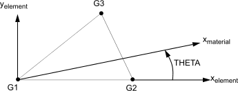
Attributes:

eid,int

Element identification number.

pid,int

Property identification number.

area,double

Element area.

alpha_shear_locking,double

Factor used to prevent shear locking, adopted from the DFG element, affecting stiffness terms E44, E45, E45:

maxl = max(edge_12, edge_23, edge_31)
factor = alpha_shear_locking*maxl**2/thickness**2
E44 = 1 / (1 + factor) * E44
# E45 = 1 / (1 + factor) * E45
E55 = 1 / (1 + factor) * E55

The adopted default is alpha_shear_locking = 0.7, based on a linear buckling analysis of a simply supported plate, such that the result approaches the one of the Quad4R element for an equivalent mesh (see the test case test_tria3r_linear_buckling_plate.py).

K6ROT,double

Dimensionless multiplier for the drilling stiffness. AUTODESK NASTRAN’s quick reference guide recommends K6ROT = 100. for static analysis. For modal solutions, K6ROT=1.e4 is suggested. MSC NASTRAN’s quick reference guide states that K6ROT > 100. should not be used, but this is contradicting AUTODESK NASTRAN.

r11, r12, r13, r21, r22, r23, r31, r32, r33double

Rotation matrix from local to global coordinates.

m11, m12, m21, m22double

Rotation matrix only for the constitutive relations. Used when a material direction is used instead of the element local coordinates.

c1, c2, c3: int

Position of each node in the global stiffness matrix.

n1, n2, n3: int

Node identification number.

init_k_KC0, init_k_KG, init_k_Mint

Position in the arrays storing the sparse data for the structural matrices.

probe,Tria3RProbe object

Pointer to the probe.

Methods

`update_KC0`(self, long[, long[, double[, ...)	Update sparse vectors for linear constitutive stiffness matrix KC0
`update_KG`(self, long[, long[, double[, ...)	Update sparse vectors for geometric stiffness matrix KG
`update_KG_given_stress`(self, double Nxx, ...)	Update sparse vectors for geometric stiffness matrix KG
`update_M`(self, long[, long[, double[, ...)	Update sparse vectors for mass matrix M
`update_area`(self)	Update element area
`update_fint`(self, double[, ShellProp prop)	Update the internal force vector
`update_probe_finte`(self, ShellProp prop)	Update the internal force vector of the probe
`update_probe_ue`(self, double[)	Update the local displacement vector of the probe of the element
`update_probe_xe`(self, double[)	Update the 3D coordinates of the probe of the element
`update_rotation_matrix`(self, double[, ...)	Update the rotation matrix of the element

K6ROT#: K6ROT: ‘double’

alpha_shear_locking#: alpha_shear_locking: ‘double’

area#: area: ‘double’

c1#: c1: ‘int’

c2#: c2: ‘int’

c3#: c3: ‘int’

eid#: eid: ‘int’

init_k_KC0#: init_k_KC0: ‘int’

init_k_KG#: init_k_KG: ‘int’

init_k_M#: init_k_M: ‘int’

m11#: m11: ‘double’

m12#: m12: ‘double’

m21#: m21: ‘double’

m22#: m22: ‘double’

n1#: n1: ‘int’

n2#: n2: ‘int’

n3#: n3: ‘int’

pid#: pid: ‘int’

probe#: probe: pyfe3d.tria3r.Tria3RProbe

r11#: r11: ‘double’

r12#: r12: ‘double’

r13#: r13: ‘double’

r21#: r21: ‘double’

r22#: r22: ‘double’

r23#: r23: ‘double’

r31#: r31: ‘double’

r32#: r32: ‘double’

r33#: r33: ‘double’

update_KC0(self, long[: :1] KC0r, long[: :1] KC0c, double[: :1] KC0v, ShellProp prop, int update_KC0v_only=0) → void#

Update sparse vectors for linear constitutive stiffness matrix KC0

Parameters:

KC0rnp.array: Array to store row positions of sparse values
KC0cnp.array: Array to store column positions of sparse values
KC0vnp.array: Array to store sparse values
propShellProp object: Shell property object from where the stiffness and mass attributes are read from.
update_KC0v_onlyint: The default 0 means that the row and column indices KC0r and KC0c should also be updated. Any other value will only update the stiffness matrix values KC0v.

update_KG(self, long[: :1] KGr, long[: :1] KGc, double[: :1] KGv, ShellProp prop, int update_KGv_only=0) → void#

Update sparse vectors for geometric stiffness matrix KG

Two-point Gauss-Legendre quadrature is used, which showed more accuracy for linear buckling load predictions.

Before this function is called, the probe Tria3RProbe attribute of the Tria3R object must be updated using update_probe_ue() with the correct pre-buckling displacements; and update_probe_xe() with the node coordinates.

Parameters:

KGrnp.array: Array to store row positions of sparse values
KGcnp.array: Array to store column positions of sparse values
KGvnp.array: Array to store sparse values
propShellProp object: Shell property object from where the stiffness and mass attributes are read from.
update_KGv_onlyint: The default \(0\) means that only \(KGv\) is updated. Any other value will lead to \(KGr\) and \(KGc\) also being updated.

update_KG_given_stress(self, double Nxx, double Nyy, double Nxy, long[: :1] KGr, long[: :1] KGc, double[: :1] KGv, int update_KGv_only=0) → void#

Update sparse vectors for geometric stiffness matrix KG

Note

A constant stress state is assumed within the element, according to the given values of \(N_{xx}, N_{yy}, N_{xy}\).

Two-point Gauss-Legendre quadrature is used, which showed more accuracy for linear buckling load predictions.

Before this function is called, the probe Tria3RProbe attribute of the Tria3R object must be updated using update_probe_xe() with the node coordinates.

Parameters:

KGrnp.array: Array to store row positions of sparse values
KGcnp.array: Array to store column positions of sparse values
KGvnp.array: Array to store sparse values
update_KGv_onlyint: The default \(0\) means that only \(KGv\) is updated. Any other value will lead to \(KGr\) and \(KGc\) also being updated.

update_M(self, long[: :1] Mr, long[: :1] Mc, double[: :1] Mv, ShellProp prop, int mtype=0) → void#

Update sparse vectors for mass matrix M

Different integration schemes are available by means of the mtype parameter.

Parameters:

Mrnp.array: Array to store row positions of sparse values
Mcnp.array: Array to store column positions of sparse values
Mvnp.array: Array to store sparse values
mtypeint, optional: 0 for consistent mass matrix using method from Brockman 1987 1 for reduced integration mass matrix using method from Brockman 1987 2 for lumped mass matrix using method from Brockman 1987

update_area(self) → void#: Update element area

update_fint(self, double[: :1] fint, ShellProp prop) → void#

Update the internal force vector

Parameters:

fintnp.array: Array that is updated in place with the internal forces. The internal forces stored in fint are calculated in global coordinates. Method update_probe_finte() is called to update the parameter finte of the Tria3RProbe with the internal forces in local coordinates.
propShellProp object: Shell property object from where the stiffness and mass attributes are read from.

update_probe_finte(self, ShellProp prop) → void#

Update the internal force vector of the probe

The attribute finte is updated with the Tria3RProbe the internal forces in local coordinates. While using this function, mind that the probe can be shared amongst more than one finite element, depending how you defined them, meaning that the probe will always safe the values from the last udpate.

Note

The finte attribute of object Tria3RProbe is updated, accessible using .probe.finte.

Parameters:

propShellProp object: Shell property object from where the stiffness and mass attributes are read from.

update_probe_ue(self, double[: :1] u) → void#

Update the local displacement vector of the probe of the element

Note

The ue attribute of object Tria3RProbe is updated, accessible using .probe.ue.

Parameters:

uarray-like: Array with global displacements, for a total of \(M\) nodes in the model, this array will be arranged as: \(u_1, v_1, w_1, {r_x}_1, {r_y}_1, {r_z}_1, u_2, v_2, w_2, {r_x}_2, {r_y}_2, {r_z}_2, ..., u_M, v_M, w_M, {r_x}_M, {r_y}_M, {r_z}_M\).

update_probe_xe(self, double[: :1] x) → void#

Update the 3D coordinates of the probe of the element

Note

The xe attribute of object Tria3RProbe is updated, accessible using .probe.xe.

Parameters:

xarray-like: Array with global nodal coordinates, for a total of \(M\) nodes in the model, this array will be arranged as: \(x_1, y_1, z_1, x_2, y_2, z_2, ..., x_M, y_M, z_M\).

update_rotation_matrix(self, double[: :1] x, double xmati=0., double xmatj=0., double xmatk=0.) → void#

Update the rotation matrix of the element

Attributes r11,r12,r13,r21,r22,r23,r31,r32,r33 are updated, corresponding to the rotation matrix from local to global coordinates.

The element coordinate system is determined, identifying the \(ijk\) components of each axis: \({x_e}_i, {x_e}_j, {x_e}_k\); \({y_e}_i, {y_e}_j, {y_e}_k\); \({z_e}_i, {z_e}_j, {z_e}_k\).

Parameters:

xarray-like: Array with global nodal coordinates, for a total of \(M\) nodes in the model, this array will be arranged as: \(x_1, y_1, z_1, x_2, y_2, z_2, ..., x_M, y_M, z_M\).
xmati, xmatj, xmatk: array-like: Vector in global coordinates representing the material direction. This vector is projected onto the plate element, thus becoming the material direction. The \(ABD\) matrix defining the constitutive behavior of the element is rotated from the material direction to the element \(x\) axis while calculating the stiffness matrices.

class pyfe3d.tria3r.Tria3RData#

Used to allocate memory for the sparse matrices.

Attributes:

KC0_SPARSE_SIZE,int: KC0_SPARSE_SIZE = 324
KG_SPARSE_SIZE,int: KG_SPARSE_SIZE = 81
M_SPARSE_SIZE,int: M_SPARSE_SIZE = 270

KC0_SPARSE_SIZE#: KC0_SPARSE_SIZE: ‘int’

KG_SPARSE_SIZE#: KG_SPARSE_SIZE: ‘int’

M_SPARSE_SIZE#: M_SPARSE_SIZE: ‘int’

class pyfe3d.tria3r.Tria3RProbe#

Probe used for local coordinates, local displacements, local stresses etc

The idea behind using a probe is to avoid allocating larger memory buffers per finite element. The memory buffers are allocated per probe, and one probe can be shared amongst many finite elements, with the information being updated and retrieved on demand.

Note

The probe can be shared amongst more than one finite element, depending on how you defined them. Mind that the probe will always safe the values from the last udpate.

Attributes:

xe,array-like: Array of size NUM_NODES*DOF//2=9 containing the nodal coordinates in the element coordinate system, in the following order \({x_e}_1, {y_e}_1, {z_e}_1, `{x_e}_2, {y_e}_2, {z_e}_2\), \({x_e}_3, {y_e}_3, {z_e}_3\).
ue,array-like: Array of size NUM_NODES*DOF=18 containing the element displacements in the following order \({u_e}_1, {v_e}_1, {w_e}_1, {{r_x}_e}_1, {{r_y}_e}_1, {{r_z}_e}_1\), \({u_e}_2, {v_e}_2, {w_e}_2, {{r_x}_e}_2, {{r_y}_e}_2, {{r_z}_e}_2\), \({u_e}_3, {v_e}_3, {w_e}_3, {{r_x}_e}_3, {{r_y}_e}_3, {{r_z}_e}_3\).
finte,array-like: Array of size NUM_NODES*DOF=18 containing the element internal forces corresponding to the degrees-of-freedom described by ue.

finte#: finte: ‘double[::1]’

ue#: ue: ‘double[::1]’

xe#: xe: ‘double[::1]’

Tria3R - Triangular element with reduced integration (pyfe3d.tria3r)#

Tria3R - Triangular element with reduced integration (`pyfe3d.tria3r`)#