Cross-sectional analysis of beams#

The beam elements BeamC and BeamLR take the cross section through the sectional stiffness matrix C of a BeamProp, which by default is built from the integrals of a rigid cross section, with the torsional stiffness GJ and the shear moduli G12 and G13, and their correction factors, given by the user, see Shell and beam properties. The module pyfe3d.vabs computes these stiffnesses, and the couplings between them, for an arbitrary cross section made of anisotropic and non-homogeneous materials, with the variational asymptotic beam sectional analysis (VABS) of Cesnik and Hodges (1997) and Yu et al. (2002, 2012): the three-dimensional elasticity problem of a slender prismatic beam is split into a two-dimensional problem over the cross section, solved here with finite elements, and a one-dimensional beam problem, governed by the resulting sectional stiffness matrix.

Steps of an analysis#

Mesh. Node coordinates \(x_2\), \(x_3\), the \(y\) and \(z\) of the beam elements, and the connectivity of 3- or 6-node triangles and 4-, 8- or 9-node quadrilaterals, numbered counter-clockwise, see CrossSection. The origin of \(x_2\), \(x_3\) is the reference axis of the beam: all results refer to it, and it need not be the centroid.
Materials. One \(6 \times 6\) material matrix per material, in its material axes, e.g. from isotropic() or orthotropic(), and per element the material index and two angles: \(\theta_1\), which orients the local axes of the element, e.g. along a wall, and the ply angle \(\theta_3\), see rotate_material().
Classical model. CrossSection.calc_stiffness() solves the warping of the cross section for the four classical strain measures, extension, twist and two bending curvatures, and condenses it into the \(4 \times 4\) stiffness Kc. This is the generalized Euler-Bernoulli model: the warping softens the rigid section, gives the Saint-Venant torsional stiffness, and populates the couplings of anisotropic sections.
Generalized Timoshenko model. The same factorization gives the first correction of the warping, driven by the derivatives of the classical strains along the beam, and the second-order energy is transformed into the \(6 \times 6\) stiffness Kt, which adds the two transverse shear strains. Its shear entries contain the shear correction factors and the location of the shear centre, which are not assumed. The theory of these two steps is in the notes of CrossSection.calc_stiffness(), and the discretization in those of the kernel _integrate of pyfe3d.vabs.
Derived quantities. The flexibilities Fc and Ft, the tension and shear centres, and, with CrossSection.calc_mass(), the mass matrix and the mass integrals of BeamProp.
Use in the beam elements. yu_to_pyfe3d() converts the matrices to the convention of pyfe3d, and beamprop_from_vabs() creates the BeamProp with the full \(6 \times 6\) matrix, see below.
Generalized Vlasov model. For thin-walled open sections, CrossSection.calc_vlasov() gives the \(5 \times 5\) stiffness Kv, which adds the restrained warping, see below.

The analysis is linear and per station: a beam whose section varies along its length needs one analysis per station.

Axes, angles and centres#

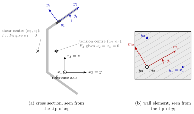
_images/vabs_axes.svg — (a) Flared channel of constant thickness, made of one isotropic material, with the tension and shear centres computed by `CrossSection.calc_stiffness()`, and an element of the upper flange with its local axes; (b) that element seen from the tip of \(y_3\), with its material axes.#

The beam axis \(x_1\) points to the viewer of the cross section and \(x_2\), \(x_3\) are the \(y\), \(z\) of BeamC and BeamLR, with the origin at the reference axis. Each element has two angles, see rotate_material():

\(\theta_1\) (theta1) rotates the local axes \(y_2\), \(y_3\) of the element about \(y_1 = x_1\), positive from \(x_2\) towards \(x_3\); for a wall, \(y_2\) is usually taken along the wall and \(y_3\) across it;
\(\theta_3\) (theta3) rotates the material axes \(m_1\), \(m_2\) about \(m_3 = y_3\), positive from \(y_1\) towards \(y_2\); for a laminated wall, it is the ply angle measured from the beam axis.

The tension centre \((a_2, a_3)\) is the point where an axial force \(F_1\) gives no bending curvature, \(\kappa_2 = \kappa_3 = 0\), and the shear centre \((e_2, e_3)\) the point where the transverse forces \(F_2\), \(F_3\) give no twist, \(\kappa_1 = 0\). Both are measured from the reference axis. For the homogeneous channel of the figure, the tension centre is the centroid and the shear centre lies outside the section, on the side of the web opposite to the flanges.

This convention of the angles reproduces all the signs of the box beam CUS computed with VABS 3.2 by Yu et al. (2012). With it, two other published examples give three couplings each with the published magnitude and the opposite sign, which is attributed to the labelling of their axes and ply angles: the box beam CAS1 of Yu et al. (2002) and the pipe of Yu and Hodges (2005), see the notes of rotate_material() and tests/test_vabs_composite.py.

Two conventions#

The matrices of CrossSection are written in the convention of the VABS literature, which orders the strains as \(\{\gamma_{11}, 2\gamma_{12}, 2\gamma_{13}, \kappa_1, \kappa_2, \kappa_3\}\) and defines the curvatures as the components of the curvature vector, i.e. the rates of rotation about \(x_1\), \(x_2\) and \(x_3\). The beam elements of pyfe3d use \(\{\bar{\varepsilon}, \bar{\gamma}_y, \bar{\gamma}_z, \kappa_x, \kappa_y, \kappa_z\}\), with \(\kappa_y\) and \(\kappa_z\) named after the coordinate they multiply in the axial strain, see the notes of BeamC. The two agree on the extension, the shear strains and the twist, while \(\kappa_2 = \kappa_z\) and \(\kappa_3 = -\kappa_y\); the moments are \(M_2 = M_y\) and \(M_3 = -M_z\). Hence, when the reference axis is offset from the centroid by \(d_2\) along \(x_2\), the coupling of the extension with \(\kappa_3\) is \(-E A d_2\) in Kt and the coupling with \(\kappa_y\) is \(E A d_2 = E Q_z\) after yu_to_pyfe3d(), as in the rigid section of BeamC; this is checked in tests/test_vabs_isotropic.py.

The ordering of the classical model is the same without the shear strains, and the classical model is recovered from the Timoshenko one by a condensation of the flexibility, classical_from_timoshenko(), not by deleting rows and columns of the stiffness.

From the sectional matrix to the beam elements#

The sectional stiffness matrix C of BeamProp has the 21 independent entries of a symmetric \(6 \times 6\) matrix, in the order of pyfe3d, i.e. C = yu_to_pyfe3d(sec.Kt):

Index of `C`	0	1	2	3	4	5
Strain of pyfe3d	\(\bar{\varepsilon}\)	\(\bar{\gamma}_y\)	\(\bar{\gamma}_z\)	\(\kappa_x\)	\(\kappa_y\)	\(\kappa_z\)
Strain of `Kt`, index	\(\gamma_{11}\), 0	\(2\gamma_{12}\), 1	\(2\gamma_{13}\), 2	\(\kappa_1\), 3	\(-\kappa_3\), 5	\(\kappa_2\), 4

beamprop_from_vabs() stores it in C, with the extension-shear, extension-twist, shear-shear, bending-shear and bending-twist couplings of a composite section, and fills the 11 parameters of the rigid section, A, E, G12, G13, GJ, Ay, Az, Iyy, Izz and Iyz, from the entries of C for information; once C is set, the elements read only C, which must be positive semi-definite, see BeamProp. With these 11 parameters alone, i.e. after del prop.C, the shear centre is the tension centre and the couplings above are lost, see the notes of BeamProp. For isotropic sections, the computed G12, G13 and GJ replace the shear correction factors and the torsion constant that the user would otherwise supply.

With couplings, BeamLR, whose linear interpolation does not depend on C, converges as the square of the element length as for an uncoupled section. BeamC derives its shape functions from the equilibrium equations of the beam with the full C, see “Shape functions with couplings” in the notes of BeamC, and is exact for nodal loads with any C, which must then be positive definite. For the box beam CUS of Yu et al. (2012), whose bending-shear couplings are strong, the tip displacements of a cantilever of length 10 in. under tip loads or moments are exact to 5.4e-16 with one element of BeamC, and have errors of 2.3e-4 with 32 elements of BeamLR, which is exact under the tip moments; the twist due to an axial load is exact with both elements and any mesh, and the natural frequencies of BeamC converge to those of BeamLR, see tests/test_beam_sectional_stiffness.py.

Generalized Vlasov model#

In a thin-walled open section, a twist rate that varies along the beam produces axial stresses through the warping, with a stiffness that can exceed the Saint-Venant GJ by far, which neither the classical nor the Timoshenko model represents. Following Yu et al. (2005), Section 2, CrossSection.calc_vlasov() moves the origin of the cross section to the shear centre with CrossSection.translated(), analyses the translated section, and keeps, in its second-order energy, only the derivative \(\kappa_1'\) of the twist rate among the derivatives of the classical strains. The result is the \(5 \times 5\) stiffness Kv of the strains \(\{\gamma_{11}, \kappa_1, \kappa_2, \kappa_3, \kappa_1'\}\) referred to the shear centre, work-conjugate to \(\{F_1, M_1, M_2, M_3, M_\omega\}\), with the bimoment \(M_\omega\); its last diagonal entry is the warping rigidity, \(E\Gamma\) for an isotropic thin-walled section:

sec.calc_vlasov()
EGamma = sec.Kv[4, 4]
w1 = sec.vlasov_section.warping([0., 1., 0., 0.])[:, 0]

The first four rows and columns are the classical stiffness about the shear centre. The model is computed by default with the warping constraints of Yu et al. (2002), constraint='yu2002', which reproduce the VABS results of Yu et al. (2005) and, for a strip, their asymptotic thin-walled warping rigidity. The constraints of Yu et al. (2012), constraint='yu2012', the default of CrossSection.calc_stiffness(), differ in the fourth constraint, on the rotation of the in-plane warping. They give the same first four rows and columns of Kv and, in the tested cases, the same shear centre, but a different warping rigidity Kv[4, 4], lower for strips and nearly equal for I- and channel sections. For the cases of tests/test_vabs_vlasov.py, with \(E = 10^7\) and \(\nu = 0.3\) for the isotropic ones:

Case	`'yu2002'`	`'yu2012'`	Reference
Isotropic strip, Table 1 of Yu et al. (2005)	1.78634	1.61715	VABS 1.78635; \(E h^3 b^3/[144(1 - \nu^2)]\) = 1.78336; \(E h^3 b^3/144\) = 1.62286
Orthotropic strip, Table 3	3.39252	3.32682	VABS 3.39251
Anisotropic strip, 15 degrees, Table 4	1.82501	1.59940	VABS 1.82499
Isotropic I-beam, Table 5, mesh of the paper	3518.92	3515.17	VABS 3553.43; thin-walled \(E t b_f^3 h^2/24\) = 3526.67
Channel, \(t = 0.01\)	912.037	911.853	thin-walled \(E \Gamma\) = 911.458

The torsional warping \(w_1\) per unit twist rate is the same for both. No beam element of pyfe3d has a warping degree-of-freedom: Kv is an output for one-dimensional Vlasov beam analyses outside pyfe3d, such as that of Section 3 of Yu et al. (2005).

Plotting the warping#

After CrossSection.calc_stiffness(), CrossSection.warping() returns the warping displacements \(w_1, w_2, w_3\) of the nodes for given strains of the beam, and CrossSection.triangles() a triangulation of the mesh through all its nodes. These two arrays are all that a plotting library needs, and pyfe3d does not depend on any. The warping satisfies the constraints chosen in CrossSection.calc_stiffness(), among them zero average, and it is the warping relative to the rigid motion of the section about the reference axis. In the tested cases, the two sets of constraints, 'yu2012' and 'yu2002', give the same out-of-plane warping per unit classical strain, but they can differ in the in-plane warping and in the term of the derivatives of the strains; CrossSection.translated() does not depend on them.

The torsional warping is therefore shown, as in the literature, about the shear centre: the section translated to the shear centre with CrossSection.translated(), as in CrossSection.calc_vlasov(), gives the warping relative to the rotation about the shear centre, with zero average. For a thin-walled open section it is the principal sectorial coordinate \(\omega\) of Vlasov (1961, Eqs. (3.15) and (7.1), pp. 14-16 and 40-41), \(\omega = \int \rho \, ds\), \(\rho\) being the distance from the pole to the tangent of the mid-line, normalised with the pole at the shear centre such that \(\omega\) has zero average and is orthogonal to \(x_2\) and \(x_3\): with \(\rho\) positive when the radius from the pole turns from \(x_2\) towards \(x_3\), the absence of shear strain on the mid-line gives \(w_1 = -\omega \kappa_1\). This is checked for a channel in tests/test_vabs_vlasov.py.

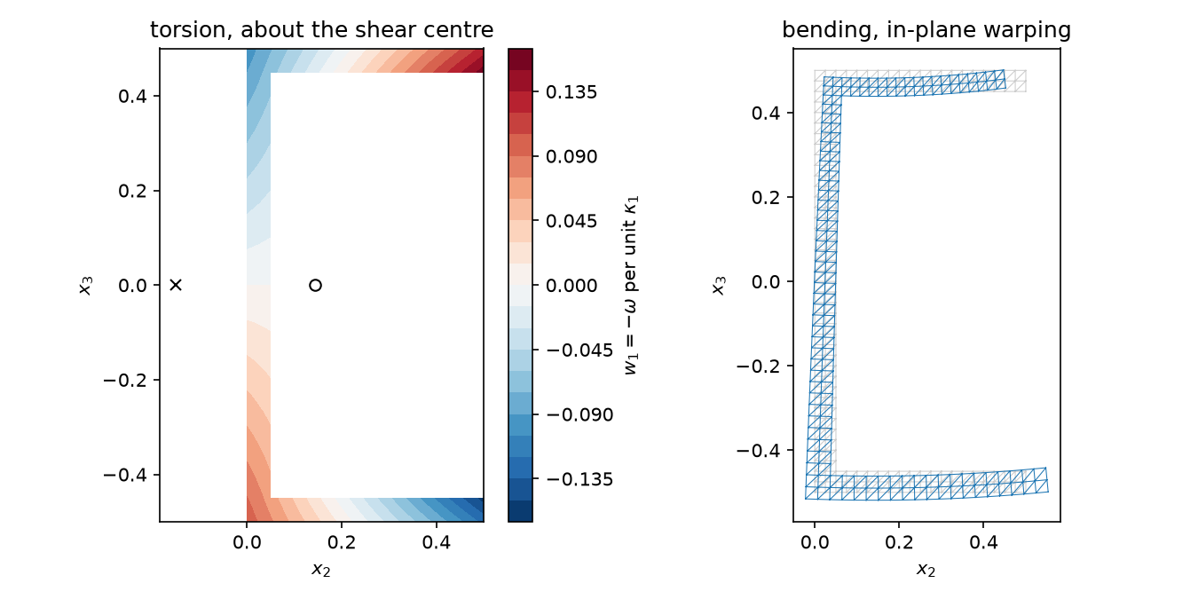
With matplotlib, for a thin-walled channel, the out-of-plane warping \(w_1\) per unit twist rate \(\kappa_1\) about the shear centre (cross), with the tension centre (circle), and the in-plane warping per unit curvature \(\kappa_2\), i.e. the anticlastic deformation due to the Poisson effect, drawn to scale on the undeformed mesh: the flange in tension, \(x_3 > 0\), contracts, and the flange in compression expands. The torsional warping is linear along each wall, \(-\omega\), and changes sign on the web, at the centre of the section, and along the flanges.

import numpy as np
import matplotlib.pyplot as plt
from matplotlib.tri import Triangulation

from pyfe3d.vabs import CrossSection, isotropic

# channel: web of height h along x3, flanges of width b along x2,
# thickness t, meshed with bilinear quadrilaterals of side t/2
h, b, t = 1., 0.5, 0.05
d = t/2
xs = np.linspace(0., b, round(b/d) + 1)
ys = np.linspace(-h/2, h/2, round(h/d) + 1)
X2, X3 = np.meshgrid(xs, ys)
nx = xs.size
elements = []
for j in range(ys.size - 1):
    for i in range(nx - 1):
        xc, yc = (xs[i] + xs[i + 1])/2, (ys[j] + ys[j + 1])/2
        if xc < t or abs(yc) > h/2 - t:
            n = j*nx + i
            elements.append([n, n + 1, n + 1 + nx, n + nx])
used = np.unique(elements)
new = -np.ones(X2.size, dtype=int)
new[used] = np.arange(used.size)
x2, x3 = X2.ravel()[used], X3.ravel()[used]
elements = new[np.array(elements)]

sec = CrossSection(x2, x3, elements, materials=[isotropic(70e9, 0.3)],
                   mat_ids=[0]*len(elements))
sec.calc_stiffness()
tri = Triangulation(sec.x2, sec.x3, sec.triangles())
# origin at the shear centre, same nodes and triangles
sc = sec.translated(*sec.shear_centre)
sc.calc_stiffness()

fig, (ax1, ax2) = plt.subplots(1, 2, figsize=(9, 4.5))
w = sc.warping([0., 1., 0., 0.])  # unit twist rate kappa1
cs = ax1.tricontourf(tri, w[:, 0], levels=21, cmap='RdBu_r')
fig.colorbar(cs, ax=ax1, label=r'$w_1 = -\omega$ per unit $\kappa_1$')
ax1.plot(*sec.tension_centre, 'ko', mfc='none')
ax1.plot(*sec.shear_centre, 'kx')
ax1.set_title('torsion, about the shear centre')

w = sec.warping([0., 0., 1., 0.])  # unit curvature kappa2
ax2.triplot(tri, color='0.8', lw=0.5)
ax2.triplot(sec.x2 + w[:, 1], sec.x3 + w[:, 2], sec.triangles(),
            color='C0', lw=0.5)
ax2.set_title('bending, in-plane warping')
for ax in (ax1, ax2):
    ax.set_aspect('equal')
    ax.set_xlabel('$x_2$')
    ax.set_ylabel('$x_3$')
fig.tight_layout()

The same arrays give a three-dimensional view with plotly. The script below draws the channel as a beam of length 3 under a uniform twist rate: the sections rotate about the shear centre and warp along the beam by \(w_1 = -\omega \kappa_1\), the warping being exaggerated and coloured by \(w_1\). The figure can be rotated, panned and zoomed:

import numpy as np
import plotly.graph_objects as go

from pyfe3d.vabs import CrossSection, isotropic

# channel: web of height h along x3, flanges of width b along x2, thickness t
h, b, t = 1., 0.5, 0.05
d = t/2
xs = np.linspace(0., b, round(b/d) + 1)
ys = np.linspace(-h/2, h/2, round(h/d) + 1)
X2, X3 = np.meshgrid(xs, ys)
nx = xs.size
elements = []
for j in range(ys.size - 1):
    for i in range(nx - 1):
        xc, yc = (xs[i] + xs[i + 1])/2, (ys[j] + ys[j + 1])/2
        if xc < t or abs(yc) > h/2 - t:
            n = j*nx + i
            elements.append([n, n + 1, n + 1 + nx, n + nx])
used = np.unique(elements)
new = -np.ones(X2.size, dtype=int)
new[used] = np.arange(used.size)
x2, x3 = X2.ravel()[used], X3.ravel()[used]
elements = new[np.array(elements)]

sec = CrossSection(x2, x3, elements, materials=[isotropic(70e9, 0.3)],
                   mat_ids=[0]*len(elements))
sec.calc_stiffness()
e2, e3 = sec.shear_centre
# warping per unit twist rate about the shear centre, -omega
sc = sec.translated(e2, e3)
sc.calc_stiffness()
w1 = sc.warping([0., 1., 0., 0.])[:, 0]
tri = sec.triangles()

# beam of length L under the uniform twist rate k1: the sections rotate by
# k1*x1 about the shear centre and warp by k1*w1 along x1, exaggerated by
# scale
L, k1, scale = 3., np.pi/(3*3.), 3.
stations = np.linspace(0., L, 31)
# NOTE edges used by one triangle only are on the boundary of the section
edges, counts = np.unique(np.sort(np.vstack((tri[:, [0, 1]], tri[:, [1, 2]],
                                             tri[:, [2, 0]])), axis=1),
                          axis=0, return_counts=True)
edges = edges[counts == 1]
nn = x2.size
X, Y, Z, C = [], [], [], []
for s in stations:
    c, si = np.cos(k1*s), np.sin(k1*s)
    X.append(s + scale*k1*w1)
    Y.append(e2 + c*(x2 - e2) - si*(x3 - e3))
    Z.append(e3 + si*(x2 - e2) + c*(x3 - e3))
    C.append(w1)
X, Y, Z, C = map(np.concatenate, (X, Y, Z, C))
faces = [tri, tri + (stations.size - 1)*nn]  # end sections
for k in range(stations.size - 1):
    a, e = edges[:, 0] + k*nn, edges[:, 1] + k*nn
    faces += [np.column_stack((a, e, e + nn)),
              np.column_stack((a, e + nn, a + nn))]
I, J, K = np.vstack(faces).T

fig = go.Figure(go.Mesh3d(x=X, y=Y, z=Z, i=I, j=J, k=K, intensity=C,
                          colorscale='RdBu_r', colorbar=dict(title='w1'),
                          lighting=dict(ambient=0.8, diffuse=0.3,
                                        specular=0., fresnel=0.)))
fig.update_layout(scene=dict(aspectmode='data', xaxis_title='x1',
                             yaxis_title='x2', zaxis_title='x3'),
                  scene_camera=dict(eye=dict(x=-1.3, y=1.5, z=0.9)),
                  height=500, margin=dict(l=0, r=0, t=0, b=0))
# fig.show()

Validation#

The tests compare the results with elasticity solutions and with published VABS results:

tests/test_vabs_isotropic.py: rectangles, circles and tubes, with the axial and bending stiffnesses, the Saint-Venant torsion constant and the shear correction factors of the elasticity solutions, Eq. (25) of Yu and Hodges (2005) for the rectangle; the isotropic square of Yu et al. (2002), the T-section of Yu and Hodges (2005), and the couplings of an offset reference axis;
tests/test_vabs_composite.py: the box beam CUS of Yu et al. (2012), reproduced to the four digits of their VABS 3.2 results, the anisotropic pipe of Yu and Hodges (2005), with its mass properties, and the box beam CAS1 of Yu et al. (2002), with the opposite signs of three couplings of the last two examples asserted explicitly, see above;
tests/test_vabs_elements.py: integration rules, shape functions, material rotation and conventions.
tests/test_beam_sectional_stiffness.py: cantilevers of BeamC and BeamLR with a coupled sectional stiffness matrix, among them the box beam CUS of Yu et al. (2012), against the closed form obtained by integrating the strains \(\boldsymbol{C}^{-1} \boldsymbol{F}(x)\), and the tangent stiffness matrix against the derivative of the internal forces.
tests/test_vabs_warping.py: the torsional warping of an ellipse against the Saint-Venant solution, and the triangulation of every element type;
tests/test_vabs_vlasov.py: the generalized Vlasov model against the VABS results of Yu et al. (2005), Tables 1, 3 and 4, isotropic, orthotropic and anisotropic strips, reproduced to five digits or more, and Table 5, isotropic I-beam, within 1 per cent for the torsional rigidity and, for the warping rigidity, about 1 per cent below, a converged difference, within 2 per cent, the grade A of MacNeal and Harder (1985); the anisotropic I-beam of Table 6, with the lay-up reconstructed from Volovoi et al. (1999), p. 1038 and Fig. 8, within 1.1 per cent for the effective torsional rigidity and 4 per cent for the warping rigidity; the composite I-beam of Hodges and Peters (2001), p. 1601, against their asymptotic thin-walled constants, with tolerances built from the neglected terms of the thin-walled theory, the free-edge factor \(1 - 0.630 t/b\) of Timoshenko and Goodier (1951), Art. 95, Eq. (161), of the flanges for the torsional rigidity, 3.45 and 2.90 per cent at 0 and 45 degrees, and \((t/b)^2\) for the warping rigidity, 1.31 per cent, plus the rounding of the printed values and data; with the walls made thinner, the differences from the thin-walled values decrease as \(t/b\) for the torsional and as \((t/b)^2\) for the warping rigidity; and the torsional warping about the shear centre of a thin-walled channel against \(-\omega\), with its warping rigidity, all with the constraints 'yu2002' and 'yu2012'.

Limitations#

Prismatic beams only: initially twisted and curved beams, whose theory is in Yu et al. (2002, 2012), are not implemented, and non-zero k1, k2, k3 of CrossSection raise NotImplementedError.
No applied loads in the sectional analysis, Yu et al. (2012), Section 5.3, and no recovery of the three-dimensional strains and stresses, although the warping is available, see CrossSection.warping().
The generalized Vlasov model is not used by any beam element of pyfe3d.

References#

Cesnik, C. E. S., and Hodges, D. H., “VABS: A New Concept for Composite Rotor Blade Cross-Sectional Modeling”, Journal of the American Helicopter Society, 42(1), pp. 27-38, 1997. https://doi.org/10.4050/JAHS.42.27

Yu, W., Hodges, D. H., Volovoi, V. V., and Cesnik, C. E. S., “On Timoshenko-like modeling of initially curved and twisted composite beams”, International Journal of Solids and Structures, 39(19), pp. 5101-5121, 2002. https://doi.org/10.1016/S0020-7683(02)00399-2

Yu, W., and Hodges, D. H., “Generalized Timoshenko Theory of the Variational Asymptotic Beam Sectional Analysis”, Journal of the American Helicopter Society, 50(1), pp. 46-55, 2005. https://doi.org/10.4050/1.3092842

Yu, W., Hodges, D. H., Volovoi, V. V., and Fuchs, E. D., “A generalized Vlasov theory for composite beams”, Thin-Walled Structures, 43(9), pp. 1493-1511, 2005. https://doi.org/10.1016/j.tws.2005.02.003

Vlasov, V. Z., Thin-Walled Elastic Beams, 2nd ed., Israel Program for Scientific Translations, Jerusalem, 1961. Translated by Y. Schechtman.

Volovoi, V. V., Hodges, D. H., Berdichevsky, V. L., and Sutyrin, V. G., “Asymptotic theory for static behavior of elastic anisotropic I-beams”, International Journal of Solids and Structures, 36(7), pp. 1017-1043, 1999. https://doi.org/10.1016/S0020-7683(97)00341-7

Hodges, D. H., and Peters, D. A., “Lateral-torsional buckling of cantilevered elastically coupled composite strip- and I-beams”, International Journal of Solids and Structures, 38(9), pp. 1585-1603, 2001. https://doi.org/10.1016/S0020-7683(00)00111-6

Timoshenko, S. P., and Goodier, J. N., Theory of Elasticity, 2nd ed., McGraw-Hill, New York, 1951.

MacNeal, R. H., and Harder, R. L., “A proposed standard set of problems to test finite element accuracy”, Finite Elements in Analysis and Design, 1(1), pp. 3-20, 1985. https://doi.org/10.1016/0168-874X(85)90003-4

Yu, W., Hodges, D. H., and Ho, J. C., “Variational asymptotic beam sectional analysis – An updated version”, International Journal of Engineering Science, 59, pp. 40-64, 2012. https://doi.org/10.1016/j.ijengsci.2012.03.006