Quad4R - Quadrilateral element with reduced integration (`pyfe3d.quad4r`)#

The Quad4R element has 6 degrees-of-freedom (DOF): \(u\), \(v\), \(w\), \(r_x\), \(r_y\), \(r_z\). All DOF are interpolated bi-linearly between the nodes, such that any of the DOF gradients can be constant over the element when the element is rectangular.

In the reduced integration scheme used, a single point at the centroid (\(\xi=\eta=0\)) and weight \(w_{ij}=4\), preventing shear locking. The hourglass control is used according to Brockman 1987, with the orthogonalised hourglass operator of his Eq. (14), which he quotes from Belytschko and Tsay 1983:

Brockman, R. A., 1987, “Dynamics of the Bilinear Mindlin Plate Element,” Int. J. Numer. Methods Eng., 24(12), pp. 2343–2356. https://onlinelibrary.wiley.com/doi/pdf/10.1002/nme.1620241208

Belytschko, T., and Tsay, C. S., 1983, “A stabilization procedure for the quadrilateral plate element with one-point quadrature,” International Journal for Numerical Methods in Engineering, 19(3), pp. 405-419. https://doi.org/10.1002/nme.1620190308

Dimensional homogeneity of the hourglass stiffnesses#

The generalized stiffnesses of Brockman’s Eqs. (16a) and (16b),

\[E^{(h)}_u = E^{(h)}_v = \frac{0.10 E t}{1 + 1/A} \qquad E^{(h)}_w = E^{(h)}_{\theta_x} = E^{(h)}_{\theta_y} = \frac{0.10 E t^3}{1 + 1/A}\]

are not dimensionally homogeneous, \(1/A\) being an inverse area, so the artificial stiffness depends on the unit of length the model is written in. The hourglass term enters the element matrix as

\[K_{ij} = A E^{(h)} \gamma_i \gamma_j\]

with \(\gamma = \partial^2 N/\partial x \partial y\) evaluated at the centroid, of dimension \(1/L^2\). The hourglass amplitude of a translation is \(\gamma^T u\), of dimension \(1/L\), and of a rotation is \(\gamma^T \theta\), of dimension \(1/L^2\). Requiring \(K_{ij}\) to be a force per unit displacement for the translations and a moment per unit rotation for the rotations gives

\[[E^{(h)}] = F L \quad \text{for } u, v, w \qquad [E^{(h)}] = F L^3 \quad \text{for } \theta_x, \theta_y\]

Since \(1/(1 + 1/A) \rightarrow A\) for \(A \ll 1\) and \(\rightarrow 1\) for \(A \gg 1\), Brockman’s factor supplies the area that Eq. (16a) is missing only in a unit of length that makes the element areas small, and stops supplying it in a unit that makes them large. The switch happens at \(A = 1\) in whatever unit is used. He introduces the factor knowingly, as “motivated by locking problems observed in elements with extremely small dimensions”, and reports good behaviour “over a range of six orders of magnitude in the planform dimension”.

This element replaces the factor by the area itself wherever doing so costs nothing, which is four of the five coefficients:

\[E^{(h)}_u = 0.10 E_{1eq} t A \qquad E^{(h)}_v = 0.10 E_{2eq} t A\]

\[E^{(h)}_{\theta_x} = 0.10 E_{2eq} t^3 A \qquad E^{(h)}_{\theta_y} = 0.10 E_{1eq} t^3 A\]

Each of these scales under a change of length unit exactly as the physical stiffness it stabilises, \(Et\) for the in-plane translations and \(Et^3\) for the rotations, so the ratio of artificial to physical stiffness is the same number in every unit. In the small-area limit they coincide with Eqs. (16a) and (16b), so no benchmark of this element moves: the change is a reinterpretation of Brockman’s factor as the area it tends to, not a different magnitude of stabilisation. Cook’s in-plane bending problem, whose response legitimately contains hourglass components, is reproduced to twelve significant figures over nine orders of magnitude of length unit, where before it drifted at the metre and collapsed at the kilometre.

The transverse coefficient \(E^{(h)}_w\) keeps Brockman’s factor, and this is a deliberate limitation rather than an oversight. The hourglass operator cannot distinguish the spurious pattern \(w = xy\) with \(\theta_x = \theta_y = 0\) from a legitimate twist curvature, since both give \(\gamma^T w = \partial^2 w/\partial x \partial y\). The stabilisation therefore also stiffens real twist, by the ratio \(3 E^{(h)}_w/(E t^3)\), and the amount that is acceptable is a property of the problem rather than of the element. Measured on this element’s own benchmarks, the thin plates want a coefficient near \(2 \times 10^{-4}\) of \(E t^3\), above which their buckling loads stiffen past their tolerances, while the one-element-wide torsion strip of MacNeal and Harder (1985), for which the twist is the hourglass pattern, wants near \(2 \times 10^{-2}\), below which it becomes several times too flexible. Those are two orders of magnitude apart and no single dimensionless constant serves both. Brockman’s factor does serve both, because it grows with the element area, which in SI units happens to correlate with which of the two regimes a given problem is in.

So the residual unit dependence of this element’s hourglass control is confined to \(E^{(h)}_w\), it is documented, and it is measured in test_quad4r_hourglass_control.py. Removing it properly needs an operator that separates the spurious transverse pattern from genuine twist, which is what an assumed-strain formulation such as MITC4 provides, rather than a better choice of coefficient.

All stiffness terms, besides drilling, are integrated using the reduced integration scheme for the Quad4R element, making it very efficient concerning the time needed to calculate the internal forces and stiffness matrices, in comparison with the pyfe3d.Quad4 element.

The transverse shear stiffnesses \(A_{44}\), \(A_{45}\) and \(A_{55}\) are read from the pyfe3d.shellprop.ShellProp object with the shear correction already applied, see pyfe3d.shellprop.ShellProp.calc_transverse_shear_stiffness(), and no shear correction factor is applied by the element. When a material direction is defined, they are brought to the element coordinate system with pyfe3d.shellprop.ShellProp.calc_Ats_element(), which re-evaluates the equilibrium-based stiffness of Rohwer (1988) with the plies rotated to the element coordinate system, such that the assumed cylindrical bending states are posed along the element axes.

Two drilling models are available, selected with the drilling_model attribute, whose default is 0:

Hughes, T. J. R., and Brezzi, F., 1989, “On drilling degrees of freedom,” Computer Methods in Applied Mechanics and Engineering, 72(1), pp. 105-121. https://doi.org/10.1016/0045-7825(89)90124-2

Allman, D. J., 1984, “A compatible triangular element including vertex rotations for plane elasticity analysis,” Computers & Structures, 19(1-2), pp. 1-8. https://doi.org/10.1016/0045-7949(84)90197-4

Both use the same operator, the regularised one of Hughes and Brezzi (1989) that ties the drilling rotation \(r_z\) to the in-plane rotation \(\theta_z = (v_{,x} - u_{,y})/2\), integrated with two points per direction, and they differ only in the coefficient \(\gamma_{r_z}\) that multiplies it:

drilling_model = 0, the default, uses the physics-based value \(\gamma_{r_z} = A_{66}\) identified by Hughes and Brezzi, which is a modulus of the laminate and not an adjustable parameter;
drilling_model = 1 uses the fictitious value \(\gamma_{r_z} = K6ROT \cdot 10^{-6} A_{66}\) of MSC Nastran and Autodesk Nastran, derived below.

Unlike pyfe3d.Quad4 and pyfe3d.Tria3R, this element does not use the hierarchical edge-mode enrichment of the in-plane displacement field of Allman (1984) that accompanies the Hughes-Brezzi term in those two elements. The enrichment exists to remove the excessive in-plane bending stiffness of the bilinear displacement field, and the single-point integration of this element already removes it: on Cook’s membrane problem, with a reference tip displacement of 23.96,

so the enrichment recovers for pyfe3d.Quad4 what the reduced integration already gives here, and adding it to this element makes it less accurate and more computationally expensive.

Integrating the enrichment consistently with the single point of the element was also evaluated and rejected. The enriched membrane operator sampled at one point supplies at most three independent rows over the twelve in-plane degrees-of-freedom, and a rectangle then keeps one spurious in-plane zero-energy mode, namely

\[u \propto x \quad , \quad v \propto -y \quad , \quad r_z \propto \pmb{h} = [1, -1, 1, -1]^\top\]

in which the uniform membrane strain of the \(u\) and \(v\) fields is exactly cancelled at the centroid by the enrichment strain of the hourglass pattern of \(r_z\). That mode escapes every term of the element: the one-point membrane term because its centroidal strain vanishes, the hourglass control of Brockman because \(u\) and \(v\) are linear fields and carry no hourglass content, and the Hughes-Brezzi term because \(r_z - \theta_z\) vanishes not only at the integration points but identically over the element, so no quadrature of that term can reach it. Removing it would require a further artificial stabilisation of the drilling rotation, of the kind this element already uses for its other degrees-of-freedom, for a change of the Cook results above of less than half a per cent.

Use pyfe3d.Quad4 to use Allman’s enrichment.

The drilling_model = 1 branch follows the approach adopted in MSC Nastran and Autodesk Nastran, using a penalty-based method. It provides a non-physical drilling stiffness with the objective of removing the singularity, by creating an artificial stiffness between the drilling rotation degree-of-freedom of each node and the in-plane rotational strain. The operator and its quadrature, two points per direction, are the same as for drilling_model = 0, only the coefficient differing. The penalty energy is defined per element as:

\[U_{drill} = \frac{1}{2} K6ROT \cdot 10^{-6} \cdot \int_A A_{66} (r_z - \theta_z)^2 dA\]

where \(10^{-6}\) is a scaling factor suggested by MSC Nastran’s approach (CQUAD4) to make the artificial drilling stiffness sufficiently small. AUTODESK NASTRAN’s quick reference guide recommends \(K6ROT = 100\) for static analysis. For modal solutions, \(K6ROT = 10^4\) is suggested. MSC NASTRAN’s quick reference guide states that \(K6ROT > 100\) should not be used, thus contradicting AUTODESK NASTRAN. The rotation \(r_z\) represents the drilling degree-of-freedom in element’s coordinates, whereas \(\theta_z\) the in-plane rotation strain, defined as:

\[\theta_z = \frac{1}{2}\left(\frac{\partial v}{\partial x} - \frac{\partial u}{\partial y}\right)\]

The first variation of U_{drill} then becomes:

\[\delta U_{drill} = K6ROT \cdot 10^{-6} \cdot \int_A A_{66} (r_z - \theta_z)(\delta r_z - \delta \theta_z) dA\]

which can be expressed in terms of the shape functions and element degrees-of-freedom (\(u_e\)) as: \(r_z = S^{r_z} u_e\), \(u = S^u u_e\) and \(v = S_v u_e\) as:

\[\delta U_{drill} = K6ROT \cdot 10^{-6} \cdot u_e^\top \int_A A_{66} (S^{r_z \top} + 1/2 S^{u \top}_{,y} - 1/2 S^{v \top}_{,x})(\delta S^{r_z} + 1/2 \delta S^u_{,y} - 1/2 S^v_{,x}) dA u_e\]

or simply as:

\[\delta U_{drill} = K6ROT \cdot 10^{-6} \cdot A_{66} u_e^\top \int_A B_{drill}^\top B_{drill} dA u_e\]

with:

\[B_{drill} = S^{r_z} + 1/2 S^u_{,y} - 1/2 S^v_{,x}\]

Note that \(A_{66}\) is assumed constant over the element, which here has no difference given that a reduced integration approach is used. The approach herein presented is very similar to the one presented in Eq. 2.20 of:

Adam, F. M., Mohamed, A. E., and Hassaballa, A. E., 2013, “Degenerated Four Nodes Shell Element with Drilling Degree of Freedom,” IOSR J. Eng., 3(8), pp. 10–20.

class pyfe3d.quad4r.Quad4R#

Nodal connectivity for the plate element similar to Nastran’s CQUAD4:

 ^ y
 |
4 ________ 3
 |       |
 |       |   --> x
 |       |
 |_______|
1         2

The element coordinate system is determined identically what is explained in Nastran’s quick reference guide for the CQUAD4 element, as illustrated below.

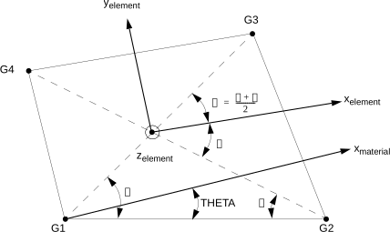
Attributes:

eid,int

Element identification number.

pid,int

Property identification number.

area,double

Element area.

drilling_model,int

Selects the coefficient of the drilling stiffness, see the module documentation. The default is 0, the physics-based \(\gamma_{r_z} = A_{66}\) of Hughes and Brezzi (1989); with anything else the fictitious penalty of MSC Nastran and Autodesk Nastran controlled by K6ROT is used instead. Both apply the same operator with the same quadrature, so switching between them changes only the magnitude of the drilling stiffness, by four orders of magnitude for the recommended K6ROT = 100..

Note that this element does not implement the in-plane enrichment of Allman (1984) that pyfe3d.Quad4 and pyfe3d.Tria3R apply together with the Hughes-Brezzi term, because its reduced integration already achieves what the enrichment achieves there, see the module documentation.

K6ROT,double

Dimensionless multiplier for the fictitious drilling stiffness, read only when drilling_model is not 0. AUTODESK NASTRAN’s quick reference guide recommends K6ROT = 100. for static analysis. For modal solutions, K6ROT=1.e4 is suggested. MSC NASTRAN’s quick reference guide states that K6ROT > 100. should not be used, but this is contradicting AUTODESK NASTRAN.

gamma_rz,double

Coefficient \(\gamma_{r_z}\) of the Hughes-Brezzi drilling stiffness, read only when drilling_model is 0. The default is a negative value, which means that \(A_{66}\) of the laminate extensional stiffness matrix is used, the value identified by Hughes and Brezzi (1989).

r11, r12, r13, r21, r22, r23, r31, r32, r33double

Rotation matrix from local to global coordinates.

m11, m12, m21, m22double

Rotation matrix only for the constitutive relations. Used when a material direction is used instead of the element local coordinates.

c1, c2, c3, c4int

Position of each node in the global stiffness matrix.

n1, n2, n3, n4int

Node identification number.

init_k_KC0, init_k_KCNL, init_k_KG, init_k_Mint

Position in the arrays storing the sparse data for the structural matrices.

init_k_KA_beta, init_k_KA_gamma, init_k_CAint

Position in the arrays storing the sparse data for the aerodynamic matrices based on the Piston theory.

probe,Quad4RProbe object

Pointer to the probe.

Methods

`update_CA`(self, long[, long[, double[)	Update sparse vectors for piston-theory aerodynamic damping matrix \(CA\)
`update_KA_beta`(self, long[, long[, double[)	Update sparse vectors for piston-theory aerodynamic matrix \(KA_{\beta}\)
`update_KA_gamma`(self, long[, long[, double[)	Update sparse vectors for piston-theory aerodynamic matrix \(KA_{\gamma}\)
`update_KC0`(self, long[, long[, double[, ...)	Update sparse vectors for linear constitutive stiffness matrix KC0
`update_KCNL`(self, long[, long[, double[, ...)	Update sparse vectors for the nonlinear constitutive stiffness matrix KCNL
`update_KG`(self, long[, long[, double[, ...)	Update sparse vectors for geometric stiffness matrix KG
`update_KG_given_stress`(self, double Nxx, ...)	Update sparse vectors for geometric stiffness matrix KG
`update_M`(self, long[, long[, double[, ...)	Update sparse vectors for mass matrix M
`update_area`(self)	Update element area
`update_fint`(self, double[, ShellProp prop, ...)	Update the internal force vector
`update_probe_finte`(self, ShellProp prop, ...)	Update the internal force vector of the probe
`update_probe_ue`(self, double[)	Update the local displacement vector of the probe of the element
`update_probe_xe`(self, double[)	Update the 3D coordinates of the probe of the element
`update_rotation_matrix`(self, double[, ...)	Update the rotation matrix of the element

K6ROT#: K6ROT: ‘double’

area#: area: ‘double’

c1#: c1: ‘int’

c2#: c2: ‘int’

c3#: c3: ‘int’

c4#: c4: ‘int’

drilling_model#: drilling_model: ‘int’

eid#: eid: ‘int’

gamma_rz#: gamma_rz: ‘double’

init_k_CA#: init_k_CA: ‘int’

init_k_KA_beta#: init_k_KA_beta: ‘int’

init_k_KA_gamma#: init_k_KA_gamma: ‘int’

init_k_KC0#: init_k_KC0: ‘int’

init_k_KCNL#: init_k_KCNL: ‘int’

init_k_KG#: init_k_KG: ‘int’

init_k_M#: init_k_M: ‘int’

m11#: m11: ‘double’

m12#: m12: ‘double’

m21#: m21: ‘double’

m22#: m22: ‘double’

n1#: n1: ‘int’

n2#: n2: ‘int’

n3#: n3: ‘int’

n4#: n4: ‘int’

pid#: pid: ‘int’

probe#: probe: pyfe3d.quad4r.Quad4RProbe

r11#: r11: ‘double’

r12#: r12: ‘double’

r13#: r13: ‘double’

r21#: r21: ‘double’

r22#: r22: ‘double’

r23#: r23: ‘double’

r31#: r31: ‘double’

r32#: r32: ‘double’

r33#: r33: ‘double’

update_CA(self, long[: :1] CAr, long[: :1] CAc, double[: :1] CAv) → void#

Update sparse vectors for piston-theory aerodynamic damping matrix \(CA\)

Parameters:

CArnp.array: Array to store row positions of sparse values
CAcnp.array: Array to store column positions of sparse values
CAvnp.array: Array to store sparse values

update_KA_beta(self, long[: :1] KA_betar, long[: :1] KA_betac, double[: :1] KA_betav) → void#

Update sparse vectors for piston-theory aerodynamic matrix \(KA_{\beta}\)

Parameters:

KA_betarnp.array: Array to store row positions of sparse values
KA_betacnp.array: Array to store column positions of sparse values
KA_betavnp.array: Array to store sparse values

update_KA_gamma(self, long[: :1] KA_gammar, long[: :1] KA_gammac, double[: :1] KA_gammav) → void#

Update sparse vectors for piston-theory aerodynamic matrix \(KA_{\gamma}\)

Parameters:

KA_gammarnp.array: Array to store row positions of sparse values
KA_gammacnp.array: Array to store column positions of sparse values
KA_gammavnp.array: Array to store sparse values

update_KC0(self, long[: :1] KC0r, long[: :1] KC0c, double[: :1] KC0v, ShellProp prop, int update_KC0v_only=0, double hgfactor_u=1., double hgfactor_v=1., double hgfactor_w=1., double hgfactor_rx=1., double hgfactor_ry=1.) → void#

Update sparse vectors for linear constitutive stiffness matrix KC0

Parameters:

KC0rnp.array: Array to store row positions of sparse values
KC0cnp.array: Array to store column positions of sparse values
KC0vnp.array: Array to store sparse values
propShellProp object: Shell property object from where the stiffness and mass attributes are read from.
update_KC0v_onlyint: The default 0 means that the row and column indices KC0r and KC0c should also be updated. Any other value will only update the stiffness matrix values KC0v.
hgfactor_u, hgfactor_v, hgfactor_w, hgfactor_rx, hgfactor_rydouble: These offer the possibility to change the default hourglass stiffnesses for each degree-of-freedom.

update_KCNL(self, long[: :1] KCNLr, long[: :1] KCNLc, double[: :1] KCNLv, ShellProp prop, int update_KCNLv_only=0) → void#

Update sparse vectors for the nonlinear constitutive stiffness matrix KCNL

Assuming that KCNL = KC0L + KCL0 + KCLL + KGNL, built from the von Karman membrane strains

\[\epsilon_{xx} = u_{,x} + \frac{1}{2} w_{,x}^2, \quad \epsilon_{yy} = v_{,y} + \frac{1}{2} w_{,y}^2, \quad \gamma_{xy} = u_{,y} + v_{,x} + w_{,x} w_{,y}\]

whose nonlinear part is \(\{\epsilon_{NL}\} = \frac{1}{2} [B_{mL}] \{u_e\}\), with \([B_{mL}]\) its variation. With \([B_m]\) and \([B_b]\) the linear membrane and bending strain-displacement matrices, \([G]\) the gradient of \(w\), and \([A]\), \([B]\) the laminate matrices:

KC0L = \([B_m]^T [A] [B_{mL}] + [B_b]^T [B] [B_{mL}]\)
KCL0 = KC0L`^T`
KCLL = \([B_{mL}]^T [A] [B_{mL}]\)
KGNL = \([G]^T [N_{NL}] [G]\), with \(\{N_{NL}\} = [A] \{\epsilon_{NL}\}\)

The first three groups are the constitutive terms coupling the linear and the nonlinear parts of the membrane strain. KGNL is geometric, carrying the stress of the nonlinear membrane strain. It is collected here so that update_KG() stays homogeneous of degree one in the displacements, which is what a linear buckling analysis needs. With it here,

\[K_T = K_{C0} + K_{CNL}(u) + K_G(u)\]

is the exact Jacobian of the internal forces of update_fint() with nonlinear=1, and a Newton-Raphson iteration built on them converges quadratically. The quadrature of update_KG() is used.

Before this function is called, the probe Quad4RProbe attribute of the Quad4R object must be updated using update_probe_ue() with the current displacements; and update_probe_xe() with the node coordinates.

Parameters:

KCNLrnp.array: Array to store row positions of sparse values
KCNLcnp.array: Array to store column positions of sparse values
KCNLvnp.array: Array to store sparse values
propShellProp object: Shell property object from where the stiffness and mass attributes are read from.
update_KCNLv_onlyint: The default 0 means that the row and column indices KCNLr and KCNLc should also be updated. Any other value will only update the stiffness matrix values KCNLv.

update_KG(self, long[: :1] KGr, long[: :1] KGc, double[: :1] KGv, ShellProp prop, int update_KGv_only=0) → void#

Update sparse vectors for geometric stiffness matrix KG

Two-point Gauss-Legendre quadrature is used, which showed more accuracy for linear buckling load predictions.

Before this function is called, the probe Quad4RProbe attribute of the Quad4R object must be updated using update_probe_ue() with the correct pre-buckling displacements; and update_probe_xe() with the node coordinates.

Parameters:

KGrnp.array: Array to store row positions of sparse values
KGcnp.array: Array to store column positions of sparse values
KGvnp.array: Array to store sparse values
propShellProp object: Shell property object from where the stiffness and mass attributes are read from.
update_KGv_onlyint: The default \(0\) means that only \(KGv\) is updated. Any other value will lead to \(KGr\) and \(KGc\) also being updated.

update_KG_given_stress(self, double Nxx, double Nyy, double Nxy, long[: :1] KGr, long[: :1] KGc, double[: :1] KGv, int update_KGv_only=0) → void#

Update sparse vectors for geometric stiffness matrix KG

Note

A constant stress state is assumed within the element, according to the given values of \(N_{xx}, N_{yy}, N_{xy}\).

Two-point Gauss-Legendre quadrature is used, which showed more accuracy for linear buckling load predictions.

Before this function is called, the probe Quad4RProbe attribute of the Quad4R object must be updated using update_probe_xe() with the node coordinates.

Parameters:

KGrnp.array: Array to store row positions of sparse values
KGcnp.array: Array to store column positions of sparse values
KGvnp.array: Array to store sparse values
update_KGv_onlyint: The default \(0\) means that only \(KGv\) is updated. Any other value will lead to \(KGr\) and \(KGc\) also being updated.

update_M(self, long[: :1] Mr, long[: :1] Mc, double[: :1] Mv, ShellProp prop, int mtype=0) → void#

Update sparse vectors for mass matrix M

Different integration schemes are available by means of the mtype parameter.

Parameters:

Mrnp.array: Array to store row positions of sparse values
Mcnp.array: Array to store column positions of sparse values
Mvnp.array: Array to store sparse values
mtypeint, optional: 0 for consistent mass matrix using method from Brockman 1987 1 for reduced integration mass matrix using method from Brockman 1987 2 for lumped mass matrix using method from Brockman 1987

update_area(self) → void#: Update element area

update_fint(self, double[: :1] fint, ShellProp prop, double hgfactor_u=1., double hgfactor_v=1., double hgfactor_w=1., double hgfactor_rx=1., double hgfactor_ry=1., int nonlinear=0) → void#

Update the internal force vector

Parameters:

fintnp.array: Array that is updated in place with the internal forces. The internal forces stored in fint are calculated in global coordinates. Method update_probe_finte() is called to update the parameter finte of the Quad4RProbe with the internal forces in local coordinates.
propShellProp object: Shell property object from where the stiffness and mass attributes are read from.
hgfactor_u, hgfactor_v, hgfactor_w, hgfactor_rx, hgfactor_rydouble: These offer the possibility to change the default hourglass stiffnesses for each degree-of-freedom.
nonlinearint: The default 0 gives the linear internal forces, KC0*u. Any other value adds the geometrically nonlinear terms of the von Karman strains, for which the exact Jacobian of the internal forces is KC0 + KCNL + KG, see update_KCNL().

update_probe_finte(self, ShellProp prop, double hgfactor_u=1., double hgfactor_v=1., double hgfactor_w=1., double hgfactor_rx=1., double hgfactor_ry=1., int nonlinear=0) → void#

Update the internal force vector of the probe

The attribute finte of the object Quad4RProbe is updated, which corresponds to the internal forces in local coordinates. While using this function, mind that the probe can be shared amongst more than one finite element, depending how you defined them, meaning that the probe will always safe the values from the last udpate.

Note

The finte attribute of object Quad4RProbe is updated, accessible using .probe.finte.

Parameters:

propShellProp object: Shell property object from where the stiffness and mass attributes are read from.
hgfactor_u, hgfactor_v, hgfactor_w, hgfactor_rx, hgfactor_rydouble: These offer the possibility to change the default hourglass stiffnesses for each degree-of-freedom.
nonlinearint: The default 0 gives the linear internal forces, KC0*u. Any other value adds the geometrically nonlinear terms of the von Karman strains, for which the exact Jacobian of the internal forces is KC0 + KCNL + KG, see update_KCNL().

update_probe_ue(self, double[: :1] u) → void#

Update the local displacement vector of the probe of the element

Note

The probe attribute of object Quad4RProbe is updated, accessible using .probe.ue.

Parameters:

uarray-like: Array with global displacements, for a total of \(M\) nodes in the model, this array will be arranged as: \(u_1, v_1, w_1, {r_x}_1, {r_y}_1, {r_z}_1, u_2, v_2, w_2, {r_x}_2, {r_y}_2, {r_z}_2, ..., u_M, v_M, w_M, {r_x}_M, {r_y}_M, {r_z}_M\).

update_probe_xe(self, double[: :1] x) → void#

Update the 3D coordinates of the probe of the element

Note

The xe attribute of object Quad4RProbe is updated, accessible using .probe.xe.

Parameters:

xarray-like: Array with global nodal coordinates, for a total of \(M\) nodes in the model, this array will be arranged as: \(x_1, y_1, z_1, x_2, y_2, z_2, ..., x_M, y_M, z_M\).

update_rotation_matrix(self, double[: :1] x, double xmati=0., double xmatj=0., double xmatk=0.) → void#

Update the rotation matrix of the element

Attributes r11,r12,r13,r21,r22,r23,r31,r32,r33 are updated, corresponding to the rotation matrix from local to global coordinates.

The element coordinate system is determined, identifying the \(ijk\) components of each axis: \({x_e}_i, {x_e}_j, {x_e}_k\); \({y_e}_i, {y_e}_j, {y_e}_k\); \({z_e}_i, {z_e}_j, {z_e}_k\).

Parameters:

xarray-like: Array with global nodal coordinates, for a total of \(M\) nodes in the model, this array will be arranged as: \(x_1, y_1, z_1, x_2, y_2, z_2, ..., x_M, y_M, z_M\).
xmati, xmatj, xmatk: array-like: Vector in global coordinates representing the material direction. This vector is projected onto the plate element, thus becoming the material direction. The \(ABD\) matrix defining the constitutive behavior of the element is rotated from the material direction to the element \(x\) axis while calculating the stiffness matrices.

class pyfe3d.quad4r.Quad4RData#

Used to allocate memory for the sparse matrices.

Attributes:

KC0_SPARSE_SIZE,int: KC0_SPARSE_SIZE = 576
KCNL_SPARSE_SIZE,int: KCNL_SPARSE_SIZE = 576
KG_SPARSE_SIZE,int: KG_SPARSE_SIZE = 144
M_SPARSE_SIZE,int: M_SPARSE_SIZE = 480
KA_BETA_SPARSE_SIZE,int: KA_BETA_SPARSE_SIZE = 144
KA_GAMMA_SPARSE_SIZE,int: KA_GAMMA_SPARSE_SIZE = 144
CA_SPARSE_SIZE,int: CA_SPARSE_SIZE = 144

CA_SPARSE_SIZE#: CA_SPARSE_SIZE: ‘int’

KA_BETA_SPARSE_SIZE#: KA_BETA_SPARSE_SIZE: ‘int’

KA_GAMMA_SPARSE_SIZE#: KA_GAMMA_SPARSE_SIZE: ‘int’

KC0_SPARSE_SIZE#: KC0_SPARSE_SIZE: ‘int’

KCNL_SPARSE_SIZE#: KCNL_SPARSE_SIZE: ‘int’

KG_SPARSE_SIZE#: KG_SPARSE_SIZE: ‘int’

M_SPARSE_SIZE#: M_SPARSE_SIZE: ‘int’

class pyfe3d.quad4r.Quad4RProbe#

Probe used for local coordinates, local displacements, local stiffness, local stresses etc…

The idea behind using a probe is to avoid allocating larger memory buffers per finite element. The memory buffers are allocated per probe, and one probe can be shared amongst many finite elements, with the information being updated and retrieved on demand.

Note

The probe can be shared amongst more than one finite element, depending on how you defined them. Mind that the probe will always safe the values from the last udpate.

Attributes:

xe,array-like: Array of size NUM_NODES*DOF//2=12 containing the nodal coordinates in the element coordinate system, in the following order \({x_e}_1, {y_e}_1, {z_e}_1, `{x_e}_2, {y_e}_2, {z_e}_2\), \({x_e}_3, {y_e}_3, {z_e}_3\), \({x_e}_4, {y_e}_4, {z_e}_4\).
ue,array-like: Array of size NUM_NODES*DOF=24 containing the element displacements in the following order \({u_e}_1, {v_e}_1, {w_e}_1, {{r_x}_e}_1, {{r_y}_e}_1, {{r_z}_e}_1\), \({u_e}_2, {v_e}_2, {w_e}_2, {{r_x}_e}_2, {{r_y}_e}_2, {{r_z}_e}_2\), \({u_e}_3, {v_e}_3, {w_e}_3, {{r_x}_e}_3, {{r_y}_e}_3, {{r_z}_e}_3\), \({u_e}_4, {v_e}_4, {w_e}_4, {{r_x}_e}_4, {{r_y}_e}_4, {{r_z}_e}_4\).
finte,array-like: Array of size NUM_NODES*DOF=24 containing the element internal forces corresponding to the degrees-of-freedom described by ue.
BLexx, BLeyy, BLgxy, BLkxx, BLkyy, BLkxyarray-like: Arrays of size NUM_NODES*DOF=24 with the rows of the linear strain-displacement matrix for the membrane strains and curvatures, at the last evaluated integration point.
Gwx, Gwyarray-like: Arrays of size NUM_NODES*DOF=24 with the rows giving \(w_{,x}\) and \(w_{,y}\), at the last evaluated integration point.
KCNLvearray-like: KCNLve: ‘double[::1]’

BLexx#: BLexx: ‘double[::1]’

BLeyy#: BLeyy: ‘double[::1]’

BLgxy#: BLgxy: ‘double[::1]’

BLkxx#: BLkxx: ‘double[::1]’

BLkxy#: BLkxy: ‘double[::1]’

BLkyy#: BLkyy: ‘double[::1]’

Gwx#: Gwx: ‘double[::1]’

Gwy#: Gwy: ‘double[::1]’

KCNLve#: KCNLve: ‘double[::1]’

finte#: finte: ‘double[::1]’

ue#: ue: ‘double[::1]’

xe#: xe: ‘double[::1]’

Quad4R - Quadrilateral element with reduced integration (pyfe3d.quad4r)#

Dimensional homogeneity of the hourglass stiffnesses#

Quad4R - Quadrilateral element with reduced integration (`pyfe3d.quad4r`)#