Tutorial: prescribed displacement at the tip of a cantilever#
A cantilever of 10 BeamC elements, clamped at \(x = 0\), whose free end is given the transverse deflection \(\delta\) with no applied load. The prescribed deflection is imposed by partitioning the degrees of freedom (dofs) into the free ones, bu, and the known ones, bk, with the prescribed values uk, see the user guide page Linear static analyses. The deflected shape and the reactions, at the tip where the deflection is prescribed and at the clamp, are compared with the
closed form of the Timoshenko beam.
The problem is solved in two ways: by the partition written by hand with SciPy, and with Analysis(..., bu=bu, uk=uk) in a single linear step.
Reference:
Bathe, K. J., Finite Element Procedures, 2nd ed., K. J. Bathe, Watertown, MA, 2014: Sec. 4.2.2, Eqs. (4.42), (4.43) and (4.45), the partition of the prescribed displacements; Sec. 1.2, Eq. (1.2), the tip deflection of a cantilever with shear deformation.
The model and the checks are those of tests/test_prescribed_displacement_linear.py, imported below.
[1]:
import os
import sys
sys.path.insert(0, os.path.join('..', '..', 'tests'))

import numpy as np
import matplotlib.pyplot as plt
from scipy.sparse import csr_matrix

from pyfe3d import DOF
from pyfe3d.solver import solve, Analysis
from test_prescribed_displacement_linear import (cantilever_prop, cantilever,
    boundary_conditions, timoshenko_cantilever, tip_force, internal_forces,
    check_reactions)
import test_prescribed_displacement_linear as tpd
Model#
Rectangular aluminium cross section, width \(b = 0.1\) m along \(y\), height \(h = 0.2\) m along \(z\), length \(L = 1\) m (\(L/h = 5\)), \(E = 70\) GPa, \(\nu = 0.3\), prescribed tip deflection \(\delta = 10\) mm along \(Z\). BeamProp applies no shear correction factor, so the factor \(k = 5/6\) of the rectangle is put in the transverse shear modulus of the bending plane \(xz\), prop.G13 \(= k G\). BeamC uses it as \(k G A\) =
G13*A, in its shear stiffness and in the shear parameter \(\alpha_z = -12 E I_{yy}/(G_{13} A
L_e^2)\) of its shape functions, with \(L_e\) the element length. The bending stiffness of the deflection \(w\) is \(E I_{yy}\), with \(I_{yy} = b h^3/12\).
[2]:
prop, L, delta = cantilever_prop()
print('A = %g m2, Iyy = %g m4, E = %g Pa, G13 = k G = %g Pa'
      % (prop.A, prop.Iyy, prop.E, prop.G13))
nodes, ncoords, elements, KC0 = cantilever(prop, L, num_elements=10)
N = KC0.shape[0]
bk, bu, uk, tip_w = boundary_conditions(N, delta)
f = np.zeros(N) # no applied load
print('N = %d dofs, %d free, %d known; uk[tip_w] = %g m'
      % (N, bu.sum(), bk.sum(), uk[tip_w]))
A = 0.02 m2, Iyy = 6.66667e-05 m4, E = 7e+10 Pa, G13 = k G = 2.24359e+10 Pa
N = 66 dofs, 59 free, 7 known; uk[tip_w] = 0.01 m
Closed form#
For a Timoshenko cantilever loaded by a tip force \(P\), the bending moment is \(M(x) = P (L - x)\) and the shear force \(Q = P\). With the rotation of the cross section \(\theta\), \(E I \theta_{,x} = M\), and the shear strain is \(\gamma = w_{,x} - \theta = P/(k G A)\). Integrating with the clamp conditions \(w(0) = \theta(0) = 0\):
At \(x = L\), \(w(L) = P \left(\frac{L^3}{3EI} + \frac{L}{kGA}\right)\), which is Eq. (1.2) of Bathe (2014). Prescribing \(w(L) = \delta\) gives the tip reaction
the Euler-Bernoulli value. The clamp reactions balance it: the force \(-P\) along \(Z\) and the moment \(M_Y = P L\), from the moment equilibrium about the clamp, \(M_Y \boldsymbol{e}_Y + (L, 0, 0) \times (0, 0, P) = \boldsymbol{0}\). In pyfe3d the rotation about \(Y\) is \(r_y = -\theta\), since the axial displacement of a point at the height \(z\) is \(u + z r_y\) (Conventions, sign conventions). The derivation is verified with SymPy by
test_closed_form_timoshenko_cantilever of the test file, run here:
[3]:
tpd.test_closed_form_timoshenko_cantilever()
P, P_EB = tip_force(delta, prop, L)
print('Timoshenko      P    = %.6e N' % P)
print('Euler-Bernoulli P_EB = %.6e N, %.2f %% larger'
      % (P_EB, 100*(P_EB/P - 1)))
print('shear/bending flexibility 3EI/(L^2 kGA) = %.4f'
      % (3*prop.E*prop.Iyy/(L**2*prop.G13*prop.A)))
Timoshenko      P    = 1.357642e+05 N
Euler-Bernoulli P_EB = 1.400000e+05 N, 3.12 % larger
shear/bending flexibility 3EI/(L^2 kGA) = 0.0312
The shear flexibility of this beam is 3.1 % of its bending flexibility, \(3 E I/(L^2 k G A) = \frac{E}{4 k G}(h/L)^2\) for the rectangle: the Euler-Bernoulli tip force is 3.1 % larger than the Timoshenko one, a difference that is visible below but small.
1. Partition by hand with SciPy#
The dofs need not be reordered: the Boolean arrays select the blocks. The free dofs solve
and the reactions follow from the second row of the partition, \(\boldsymbol{K}_{{C0}_{ku}} \boldsymbol{u}_u + \boldsymbol{K}_{{C0}_{kk}} \boldsymbol{u}_k - \boldsymbol{f}_k\), equal to the internal forces of update_fint at the known dofs minus the loads applied there, \(\boldsymbol{F}_{{int}_k} - \boldsymbol{f}_k\). These are Eqs. (4.43) and (4.45) of Bathe (2014), with the known set written \(k\), as in pyfe3d.
[4]:
KC0uu = KC0[bu, :][:, bu]
KC0uk = KC0[bu, :][:, bk]
KC0ku = KC0[bk, :][:, bu]
KC0kk = KC0[bk, :][:, bk]

u = np.zeros(N)
u[bk] = uk[bk]
u[bu] = solve(KC0uu, f[bu] - KC0uk @ uk[bk])

R_partition = KC0ku @ u[bu] + KC0kk @ uk[bk] - f[bk]
R = internal_forces(elements, prop, u, ncoords) - f
assert np.allclose(R[bk], R_partition, rtol=1e-12, atol=1e-12*P*L)

print('tip reaction  FE %.10e N, closed form %.10e N, rel. diff. %.1e'
      % (R[tip_w], P, abs(R[tip_w]/P - 1)))
print('clamp forces  [N]   ', R[0:3])
print('clamp moments [N m] ', R[3:6], ' P L =', P*L)
check_reactions(R, nodes, L, P, rtol=1e-9)
tip reaction  FE 1.3576415826e+05 N, closed form 1.3576415826e+05 N, rel. diff. 1.4e-14
clamp forces  [N]    [      0.               0.         -135764.15826221]
clamp moments [N m]  [     0.         135764.15826222      0.        ]  P L = 135764.1582622188
check_reactions asserts, with a relative tolerance of \(10^{-9}\), the tip reaction \(P\), the clamp force \((0, 0, -P)\), the clamp moment \(M_Y = P L\) with the moment equilibrium of all the reactions about the origin, and zero forces at the free dofs. BeamC solves the homogeneous equations of the Timoshenko beam exactly, so the agreement is to round-off.
The deflected shape: the nodal deflections and rotations against the closed form, with the tolerance \(10^{-10} \delta\), and \(w(x)\) plotted with the Euler-Bernoulli shape of the same tip deflection, \(w_{EB}(x) = \delta \left(\frac{3 x^2}{2 L^2} - \frac{x^3}{2 L^3}\right)\).
[5]:
w_ref, theta_ref = timoshenko_cantilever(nodes, P, prop, L)
w_fe = u[2::DOF]
ry_fe = u[4::DOF]
print('max |w_FE - w| / delta          = %.1e' % (abs(w_fe - w_ref).max()/delta))
print('max |r_y,FE + theta| / theta(L) = %.1e'
      % (abs(ry_fe + theta_ref).max()/theta_ref[-1]))
assert np.allclose(w_fe, w_ref, rtol=0, atol=1e-10*delta)
assert np.allclose(ry_fe, -theta_ref, rtol=0, atol=1e-10*theta_ref[-1])

xs = np.linspace(0, L, 201)
w_cf, _ = timoshenko_cantilever(xs, P, prop, L)
w_eb = delta*(3*xs**2/(2*L**2) - xs**3/(2*L**3))
fig, ax = plt.subplots(figsize=(6, 4))
ax.plot(xs, 1e3*w_cf, 'k-', label='Timoshenko, closed form')
ax.plot(xs, 1e3*w_eb, 'k--', lw=1, label='Euler-Bernoulli, same $\\delta$')
ax.plot(nodes, 1e3*w_fe, 'o', mfc='none', label='BeamC, 10 elements')
ax.set_xlabel('$x$ [m]')
ax.set_ylabel('$w$ [mm]')
ax.grid(True, alpha=0.3)
ax.legend()
plt.tight_layout()
plt.show()

i = np.argmax(abs(w_cf - w_eb))
print('largest difference Timoshenko - Euler-Bernoulli: %.3f mm at x = %.2f m'
      % (1e3*(w_cf - w_eb)[i], xs[i]))
max |w_FE - w| / delta          = 2.2e-15
max |r_y,FE + theta| / theta(L) = 7.4e-15
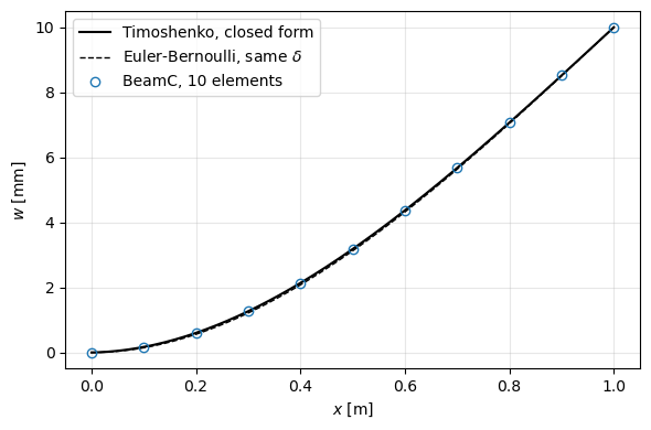
largest difference Timoshenko - Euler-Bernoulli: 0.058 mm at x = 0.42 m
2. Analysis with bu and uk#
Analysis receives the callables of the full model and the partition: the known dofs are those of ~bu, with the prescribed values uk[~bu], imposed exactly. The linear analysis, static(NLgeom=False), solves the same system \(\boldsymbol{K}_{{C0}_{uu}} \boldsymbol{u}_u = \boldsymbol{f}_u - \boldsymbol{K}_{{C0}_{uk}} \boldsymbol{u}_k\) in a single step and returns cs[0] of size N, with the prescribed values at the known dofs. calc_fext returns zeros: the analysis is
displacement controlled. The reactions are calc_fint(u) - calc_fext() at the known dofs.
[6]:
def calc_fext(inc=1., silent=True):
    return np.zeros(N)

def calc_kC(c=None, NLgeom=False, silent=True):
    return KC0

def calc_fint(c, silent=True):
    return internal_forces(elements, prop, c, ncoords)

def calc_kG(c=None, NLgeom=False, silent=True):
    return csr_matrix((N, N)) # not used by the linear analysis

an = Analysis(calc_fext, calc_fint, calc_kC, calc_kG, bu=bu, uk=uk)
increments, cs = an.static(NLgeom=False, silent=True)
u_an = cs[0]
print('increments', increments, ', u[tip_w] =', u_an[tip_w])
print('max |u_Analysis - u_partition| / delta = %.1e'
      % (abs(u_an - u).max()/delta))
assert np.allclose(u_an, u, rtol=1e-12, atol=1e-14*delta)
R_an = calc_fint(u_an) - calc_fext()
print('tip reaction %.10e N' % R_an[tip_w])
check_reactions(R_an, nodes, L, P, rtol=1e-9)
increments [1.0] , u[tip_w] = 0.01
max |u_Analysis - u_partition| / delta = 8.7e-15
tip reaction 1.3576415826e+05 N
Both ways give the closed form to round-off. The same bu and uk serve the geometrically non-linear analyses, static(NLgeom=True), where the prescribed displacements grow with the load factor, \(\lambda \boldsymbol{u}_k\), see Non-linear static analyses.
The checks are also run as tests:
[7]:
tpd.test_partition_by_hand()
tpd.test_analysis_bu_uk()
print('tests passed')
P = 1.3576415826e+05, FE 1.3576415826e+05, Euler-Bernoulli 1.4000000000e+05
tests passed