Strain-displacement (kinematic) equations for plates, cylindrical and spherical shells March 25, 2026
The discussion presented by Castro Castro, 2015 Castro, 2025 γ i j = 2 ε i j \gamma_{ij}=2\varepsilon_{ij} γ ij = 2 ε ij
1 General strain-displacement relations ¶ According to the three-dimensional (3D) elasticity theory, the strain components referred to an arbitrary orthogonal coordinate system x 1 x_1 x 1 x 2 x_2 x 2 x 3 x_3 x 3 Figure 1
Figure 1: Complete stress state of a material point.
can be written as Castro, 2015
ϵ 11 = 1 2 ( ( e 13 2 − ω 2 ) 2 + ( e 12 2 + ω 3 ) 2 + e 11 2 ) + e 11 ϵ 22 = 1 2 ( ( e 23 2 + ω 1 ) 2 + ( e 12 2 − ω 3 ) 2 + e 22 2 ) + e 22 ϵ 33 = 1 2 ( ( e 23 2 − ω 1 ) 2 + ( e 13 2 + ω 2 ) 2 + e 33 2 ) + e 33 ϵ 12 = ( e 23 2 + ω 1 ) ( e 13 2 − ω 2 ) + e 11 ( e 12 2 − ω 3 ) + e 22 ( e 12 2 + ω 3 ) + e 12 ϵ 13 = e 33 ( e 13 2 − ω 2 ) + e 11 ( e 13 2 + ω 2 ) + ( e 23 2 − ω 1 ) ( e 12 2 + ω 3 ) + e 13 ϵ 23 = e 22 ( e 23 2 − ω 1 ) + e 33 ( e 23 2 + ω 1 ) + ( e 13 2 + ω 2 ) ( e 12 2 − ω 3 ) + e 23 \begin{split}
\epsilon_{11} = \frac{1}{2}\left( \left( \frac{e_{13}}{2} - \omega_{2} \right)^{2} + \left( \frac{e_{12}}{2} + \omega_{3} \right)^{2} + e_{11}^{2} \right) + e_{11} \\
\epsilon_{22} = \frac{1}{2}\left( \left( \frac{e_{23}}{2} + \omega_{1} \right)^{2} + \left( \frac{e_{12}}{2} - \omega_{3} \right)^{2} + e_{22}^{2} \right) + e_{22} \\
\epsilon_{33} = \frac{1}{2}\left( \left( \frac{e_{23}}{2} - \omega_{1} \right)^{2} + \left( \frac{e_{13}}{2} + \omega_{2} \right)^{2} + e_{33}^{2} \right) + e_{33} \\
\epsilon_{12} = \left( \frac{e_{23}}{2} + \omega_{1} \right) \left( \frac{e_{13}}{2} - \omega_{2} \right) + e_{11} \left( \frac{e_{12}}{2} - \omega_{3} \right) + e_{22} \left( \frac{e_{12}}{2} + \omega_{3} \right) + e_{12} \\
\epsilon_{13} = e_{33} \left( \frac{e_{13}}{2} - \omega_{2} \right) + e_{11} \left( \frac{e_{13}}{2} + \omega_{2} \right) + \left( \frac{e_{23}}{2} - \omega_{1} \right) \left( \frac{e_{12}}{2} + \omega_{3} \right) + e_{13} \\
\epsilon_{23} = e_{22} \left( \frac{e_{23}}{2} - \omega_{1} \right) + e_{33} \left( \frac{e_{23}}{2} + \omega_{1} \right) + \left( \frac{e_{13}}{2} + \omega_{2} \right) \left( \frac{e_{12}}{2} - \omega_{3} \right) + e_{23}
\end{split} ϵ 11 = 2 1 ( ( 2 e 13 − ω 2 ) 2 + ( 2 e 12 + ω 3 ) 2 + e 11 2 ) + e 11 ϵ 22 = 2 1 ( ( 2 e 23 + ω 1 ) 2 + ( 2 e 12 − ω 3 ) 2 + e 22 2 ) + e 22 ϵ 33 = 2 1 ( ( 2 e 23 − ω 1 ) 2 + ( 2 e 13 + ω 2 ) 2 + e 33 2 ) + e 33 ϵ 12 = ( 2 e 23 + ω 1 ) ( 2 e 13 − ω 2 ) + e 11 ( 2 e 12 − ω 3 ) + e 22 ( 2 e 12 + ω 3 ) + e 12 ϵ 13 = e 33 ( 2 e 13 − ω 2 ) + e 11 ( 2 e 13 + ω 2 ) + ( 2 e 23 − ω 1 ) ( 2 e 12 + ω 3 ) + e 13 ϵ 23 = e 22 ( 2 e 23 − ω 1 ) + e 33 ( 2 e 23 + ω 1 ) + ( 2 e 13 + ω 2 ) ( 2 e 12 − ω 3 ) + e 23 where the parameters ϵ i j \epsilon_ij ϵ i j ω i \omega_i ω i ∂ / ∂ x \partial/\partial x ∂ / ∂ x Castro (2015) u u u v v v w w w x 1 x_1 x 1 x 2 x_2 x 2 x 3 x_3 x 3
e 11 = 1 H 1 ∂ u ∂ x 1 + v H 1 H 2 ∂ H 1 ∂ x 2 + w H 1 H 3 ∂ H 1 ∂ x 3 e 22 = u H 1 H 2 ∂ H 2 ∂ x 1 + 1 H 2 ∂ v ∂ x 2 + w H 2 H 3 ∂ H 2 ∂ x 3 e 33 = u H 1 H 3 ∂ H 3 ∂ x 1 + v H 2 H 3 ∂ H 3 ∂ x 2 + 1 H 3 ∂ w ∂ x 3 e 12 = H 1 H 2 ∂ ∂ x 2 ( u H 1 ) + H 2 H 1 ∂ ∂ x 1 ( v H 2 ) e 13 = H 1 H 3 ∂ ∂ x 3 ( u H 1 ) + H 3 H 1 ∂ ∂ x 1 ( w H 3 ) e 23 = H 2 H 3 ∂ ∂ x 3 ( v H 2 ) + H 3 H 2 ∂ ∂ x 2 ( w H 3 ) ω 1 = ∂ ( H 3 w ) ∂ x 2 − ∂ ( H 2 v ) ∂ x 3 2 ( H 2 H 3 ) ω 2 = ∂ ( H 1 u ) ∂ x 3 − ∂ ( H 3 w ) ∂ x 1 2 ( H 1 H 3 ) ω 3 = ∂ ( H 2 v ) ∂ x 1 − ∂ ( H 1 u ) ∂ x 2 2 ( H 1 H 2 ) H 1 = ( X 1 , x 1 ) 2 + ( X 2 , x 1 ) 2 + ( X 3 , x 1 ) 2 H 2 = ( X 1 , x 2 ) 2 + ( X 2 , x 2 ) 2 + ( X 3 , x 2 ) 2 H 3 = ( X 1 , x 3 ) 2 + ( X 2 , x 3 ) 2 + ( X 3 , x 3 ) 2 \begin{split}
e_{11} = \frac{1}{H_{1}}\frac{\partial u}{\partial x_{1}} + \frac{v}{H_{1}H_{2}} \frac{\partial H_{1}}{\partial x_{2}} + \frac{w}{H_{1}H_{3}} \frac{\partial H_{1}}{\partial x_{3}} \\
e_{22} = \frac{u}{H_{1}H_{2}} \frac{\partial H_{2}}{\partial x_{1}} + \frac{1}{H_{2}}\frac{\partial v}{\partial x_{2}} + \frac{w}{H_{2}H_{3}} \frac{\partial H_{2}}{\partial x_{3}} \\
e_{33} = \frac{u}{H_{1}H_{3}} \frac{\partial H_{3}}{\partial x_{1}} + \frac{v}{H_{2}H_{3}} \frac{\partial H_{3}}{\partial x_{2}} + \frac{1}{H_{3}}\frac{\partial w}{\partial x_{3}} \\
e_{12} = \frac{H_{1}}{H_{2}}\frac{\partial}{\partial x_{2}}\left(\frac{u}{H_{1}}\right) + \frac{H_{2}}{H_{1}}\frac{\partial}{\partial x_{1}}\left(\frac{v}{H_{2}}\right) \\
e_{13} = \frac{H_{1}}{H_{3}} \frac{\partial}{\partial x_{3}}\left(\frac{u}{H_{1}}\right) + \frac{H_{3}}{H_{1}} \frac{\partial}{\partial x_{1}}\left(\frac{w}{H_{3}}\right)\\
e_{23} = \frac{H_{2}}{H_{3}} \frac{\partial}{\partial x_{3}}\left(\frac{v}{H_{2}}\right) + \frac{H_{3}}{H_{2}} \frac{\partial}{\partial x_{2}}\left(\frac{w}{H_{3}}\right) \\
\omega_{1} = \frac{\frac{\partial (H_{3}w)}{\partial x_{2}} - \frac{\partial (H_{2}v)}{\partial x_{3}}}{2(H_{2}H_{3})} \\
\omega_{2} = \frac{\frac{\partial (H_{1}u)}{\partial x_{3}} - \frac{\partial (H_{3}w)}{\partial x_{1}}}{2(H_{1}H_{3})} \\
\omega_{3} = \frac{\frac{\partial (H_{2}v)}{\partial x_{1}} - \frac{\partial (H_{1}u)}{\partial x_{2}}}{2(H_{1}H_{2})} \\
H_{1} = \sqrt{(X_{1,x_{1}})^{2} + (X_{2,x_{1}})^{2} + (X_{3,x_{1}})^{2}} \\
H_{2} = \sqrt{(X_{1,x_{2}})^{2} + (X_{2,x_{2}})^{2} + (X_{3,x_{2}})^{2}} \\
H_{3} = \sqrt{(X_{1,x_{3}})^{2} + (X_{2,x_{3}})^{2} + (X_{3,x_{3}})^{2}}
\end{split} e 11 = H 1 1 ∂ x 1 ∂ u + H 1 H 2 v ∂ x 2 ∂ H 1 + H 1 H 3 w ∂ x 3 ∂ H 1 e 22 = H 1 H 2 u ∂ x 1 ∂ H 2 + H 2 1 ∂ x 2 ∂ v + H 2 H 3 w ∂ x 3 ∂ H 2 e 33 = H 1 H 3 u ∂ x 1 ∂ H 3 + H 2 H 3 v ∂ x 2 ∂ H 3 + H 3 1 ∂ x 3 ∂ w e 12 = H 2 H 1 ∂ x 2 ∂ ( H 1 u ) + H 1 H 2 ∂ x 1 ∂ ( H 2 v ) e 13 = H 3 H 1 ∂ x 3 ∂ ( H 1 u ) + H 1 H 3 ∂ x 1 ∂ ( H 3 w ) e 23 = H 3 H 2 ∂ x 3 ∂ ( H 2 v ) + H 2 H 3 ∂ x 2 ∂ ( H 3 w ) ω 1 = 2 ( H 2 H 3 ) ∂ x 2 ∂ ( H 3 w ) − ∂ x 3 ∂ ( H 2 v ) ω 2 = 2 ( H 1 H 3 ) ∂ x 3 ∂ ( H 1 u ) − ∂ x 1 ∂ ( H 3 w ) ω 3 = 2 ( H 1 H 2 ) ∂ x 1 ∂ ( H 2 v ) − ∂ x 2 ∂ ( H 1 u ) H 1 = ( X 1 , x 1 ) 2 + ( X 2 , x 1 ) 2 + ( X 3 , x 1 ) 2 H 2 = ( X 1 , x 2 ) 2 + ( X 2 , x 2 ) 2 + ( X 3 , x 2 ) 2 H 3 = ( X 1 , x 3 ) 2 + ( X 2 , x 3 ) 2 + ( X 3 , x 3 ) 2 2 3D kinematic equations for plates ¶ Figure 2
Figure 2: Plate domain.
from where the following coordinate relations can be obtained:
x 1 = x X 1 = x x 2 = y X 2 = y x 3 = z X 3 = z \begin{split}
x_{1} = x \quad X_{1} = x \\
x_{2} = y \quad X_{2} = y \\
x_{3} = z \quad X_{3} = z
\end{split} x 1 = x X 1 = x x 2 = y X 2 = y x 3 = z X 3 = z Defining:
ε x x = ϵ 11 γ x y = 2 ε x y = ϵ 12 ε y y = ϵ 22 γ x z = 2 ε x z = ϵ 13 ε z z = ϵ 33 γ y z = 2 ε y z = ϵ 23 \begin{split}
\varepsilon_{xx} = \epsilon_{11} \quad \gamma_{xy} = 2\varepsilon_{xy} = \epsilon_{12} \\
\varepsilon_{yy} = \epsilon_{22} \quad \gamma_{xz} = 2\varepsilon_{xz} = \epsilon_{13} \\
\varepsilon_{zz} = \epsilon_{33} \quad \gamma_{yz} = 2\varepsilon_{yz} = \epsilon_{23}
\end{split} ε xx = ϵ 11 γ x y = 2 ε x y = ϵ 12 ε yy = ϵ 22 γ x z = 2 ε x z = ϵ 13 ε zz = ϵ 33 γ yz = 2 ε yz = ϵ 23 We have that:
ε x x = u , x + 1 2 ( u , x 2 + v , x 2 + w , x 2 ) ε y y = v , y + 1 2 ( u , y 2 + v , y 2 + w , y 2 ) ε z z = w , z + 1 2 ( u , z 2 + v , z 2 + w , z 2 ) γ x y = u , y + v , x + ( u , x u , y + v , x v , y + w , x w , y ) γ x z = u , z + w , x + ( u , x u , z + v , x v , z + w , x w , z ) γ y z = v , z + w , y + ( u , y u , z + v , y v , z + w , y w , z ) \begin{split}
\varepsilon_{xx} = u_{,x} + \frac{1}{2}(u_{,x}^{2} + v_{,x}^{2} + w_{,x}^{2}) \\
\varepsilon_{yy} = v_{,y} + \frac{1}{2}(u_{,y}^{2} + v_{,y}^{2} + w_{,y}^{2}) \\
\varepsilon_{zz} = w_{,z} + \frac{1}{2}(u_{,z}^{2} + v_{,z}^{2} + w_{,z}^{2}) \\
\gamma_{xy} = u_{,y} + v_{,x} + (u_{,x}u_{,y} + v_{,x}v_{,y} + w_{,x}w_{,y}) \\
\gamma_{xz} = u_{,z} + w_{,x} + (u_{,x}u_{,z} + v_{,x}v_{,z} + w_{,x}w_{,z}) \\
\gamma_{yz} = v_{,z} + w_{,y} + (u_{,y}u_{,z} + v_{,y}v_{,z} + w_{,y}w_{,z})
\end{split} ε xx = u , x + 2 1 ( u , x 2 + v , x 2 + w , x 2 ) ε yy = v , y + 2 1 ( u , y 2 + v , y 2 + w , y 2 ) ε zz = w , z + 2 1 ( u , z 2 + v , z 2 + w , z 2 ) γ x y = u , y + v , x + ( u , x u , y + v , x v , y + w , x w , y ) γ x z = u , z + w , x + ( u , x u , z + v , x v , z + w , x w , z ) γ yz = v , z + w , y + ( u , y u , z + v , y v , z + w , y w , z ) 3 3D kinematic equations for cylindrical shells ¶ Figure 3
Figure 3: Cylindrical shell domain.
from where the following geometric relations can be derived Castro, 2015
x 1 = x X 1 = R ( z ) cos ( θ ) x 2 = θ X 2 = R ( z ) sin ( θ ) x 3 = z X 3 = − x \begin{split}
x_{1} = x \quad X_{1} = R(z) \cos(\theta) \\
x_{2} = \theta \quad X_{2} = R(z) \sin(\theta) \\
x_{3} = z \quad X_{3} = -x
\end{split} x 1 = x X 1 = R ( z ) cos ( θ ) x 2 = θ X 2 = R ( z ) sin ( θ ) x 3 = z X 3 = − x Defining:
ε x x = ϵ 11 γ x θ = 2 ε x θ = ϵ 12 ε θ θ = ϵ 22 γ x z = 2 ε x z = ϵ 13 ε z z = ϵ 33 γ θ z = 2 ε θ z = ϵ 23 \begin{split}
\varepsilon_{xx} = \epsilon_{11} \quad \gamma_{x\theta} = 2\varepsilon_{x\theta} = \epsilon_{12} \\
\varepsilon_{\theta\theta} = \epsilon_{22} \quad \gamma_{xz} = 2\varepsilon_{xz} = \epsilon_{13} \\
\varepsilon_{zz} = \epsilon_{33} \quad \gamma_{\theta z} = 2\varepsilon_{\theta z} = \epsilon_{23}
\end{split} ε xx = ϵ 11 γ x θ = 2 ε x θ = ϵ 12 ε θθ = ϵ 22 γ x z = 2 ε x z = ϵ 13 ε zz = ϵ 33 γ θ z = 2 ε θ z = ϵ 23 we have that, considering only the linear terms :
ε x x = u , x ε θ θ = v , θ R ( z ) + w R ( z ) ε z z = w , z γ x θ = u , θ R ( z ) + v , x γ x z = u , z + w , x γ θ z = v , z + w , θ R ( z ) − v R ( z ) \begin{split}
\varepsilon_{xx} = u_{,x} \\
\varepsilon_{\theta\theta} = \frac{v_{,\theta}}{R(z)} + \frac{w}{R(z)} \\
\varepsilon_{zz} = w_{,z} \\
\gamma_{x\theta} = \frac{u_{,\theta}}{R(z)} + v_{,x} \\
\gamma_{xz} = u_{,z} + w_{,x} \\
\gamma_{\theta z} = v_{,z} + \frac{w_{,\theta}}{R(z)} - \frac{v}{R(z)}
\end{split} ε xx = u , x ε θθ = R ( z ) v , θ + R ( z ) w ε zz = w , z γ x θ = R ( z ) u , θ + v , x γ x z = u , z + w , x γ θ z = v , z + R ( z ) w , θ − R ( z ) v These equations represent the linear part of the strain-displacement relations (small strain/small displacement). The terms containing R ( z ) R(z) R ( z ) w R ( z ) \frac{w}{R(z)} R ( z ) w ε θ θ \varepsilon_{\theta\theta} ε θθ
4 3D kinematic equations for conical shells ¶ Figure 4 Castro et al. , 2014 Castro et al. , 2015 Castro et al. , 2015 Castro, 2015
Figure 4: Conical shell domain.
from where the following geometric relations can be derived Castro, 2015
x 1 = x X 1 = R ( x , z ) cos θ x 2 = θ X 2 = R ( x , z ) sin θ x 3 = z X 3 = z sin α − x cos α R ( x , z ) = R 2 + x sin α + z cos α \begin{split}
x_{1} = x \quad X_{1} = R(x, z) \cos \theta \\
x_{2} = \theta \quad X_{2} = R(x, z) \sin \theta \\
x_{3} = z \quad X_{3} = z \sin \alpha - x \cos \alpha \\
R(x,z) = R_2 + x \sin \alpha + z \cos \alpha
\end{split} x 1 = x X 1 = R ( x , z ) cos θ x 2 = θ X 2 = R ( x , z ) sin θ x 3 = z X 3 = z sin α − x cos α R ( x , z ) = R 2 + x sin α + z cos α Defining:
ε x x = ϵ 11 γ x θ = 2 ε x θ = ϵ 12 ε θ θ = ϵ 22 γ x z = 2 ε x z = ϵ 13 ε z z = ϵ 33 γ θ z = 2 ε θ z = ϵ 23 \begin{split}
\varepsilon_{xx} = \epsilon_{11} \quad \gamma_{x\theta} = 2\varepsilon_{x\theta} = \epsilon_{12} \\
\varepsilon_{\theta\theta} = \epsilon_{22} \quad \gamma_{xz} = 2\varepsilon_{xz} = \epsilon_{13} \\
\varepsilon_{zz} = \epsilon_{33} \quad \gamma_{\theta z} = 2\varepsilon_{\theta z} = \epsilon_{23}
\end{split} ε xx = ϵ 11 γ x θ = 2 ε x θ = ϵ 12 ε θθ = ϵ 22 γ x z = 2 ε x z = ϵ 13 ε zz = ϵ 33 γ θ z = 2 ε θ z = ϵ 23 we have that, considering only the linear terms :
ε x x = u , x ε θ θ = v , θ R ( x , z ) + u sin α R ( x , z ) + w cos α R ( x , z ) ε z z = w , z γ x θ = u , θ R ( x , z ) + v , x − v sin α R ( x , z ) γ x z = w , x + u , z γ θ z = w , θ R ( x , z ) + v , z − v cos α R ( x , z ) \begin{split}
\varepsilon_{xx} = u_{,x} \\
\varepsilon_{\theta\theta} = \frac{v_{,\theta}}{R(x, z)} + \frac{u \sin \alpha}{R(x, z)} + \frac{w \cos \alpha}{R(x, z)} \\
\varepsilon_{zz} = w_{,z} \\
\gamma_{x\theta} = \frac{u_{,\theta}}{R(x, z)} + v_{,x} - \frac{v \sin \alpha}{R(x, z)} \\
\gamma_{xz} = w_{,x} + u_{,z} \\
\gamma_{\theta z} = \frac{w_{,\theta}}{R(x, z)} + v_{,z} - \frac{v \cos \alpha}{R(x, z)}
\end{split} ε xx = u , x ε θθ = R ( x , z ) v , θ + R ( x , z ) u sin α + R ( x , z ) w cos α ε zz = w , z γ x θ = R ( x , z ) u , θ + v , x − R ( x , z ) v sin α γ x z = w , x + u , z γ θ z = R ( x , z ) w , θ + v , z − R ( x , z ) v cos α The sin α \sin \alpha sin α cos α \cos \alpha cos α
5 3D kinematic equations for spherical shells ¶ Figure 5
Figure 5: Spherical shell domain.
from where the following geometric relations can be derived:
x 1 = ϕ X 1 = R ( z ) cos ϕ cos θ x 2 = θ X 2 = R ( z ) sin ϕ cos θ x 3 = z X 3 = R ( z ) sin θ R ( z ) = r + z \begin{split}
x_{1} = \phi \quad X_{1} = R(z) \cos \phi \cos \theta \\
x_{2} = \theta \quad X_{2} = R(z) \sin \phi \cos \theta \\
x_{3} = z \quad X_{3} = R(z) \sin \theta \\
R(z) = r + z
\end{split} x 1 = ϕ X 1 = R ( z ) cos ϕ cos θ x 2 = θ X 2 = R ( z ) sin ϕ cos θ x 3 = z X 3 = R ( z ) sin θ R ( z ) = r + z where ϕ \phi ϕ θ \theta θ R R R z z z
ε ϕ ϕ = ϵ 11 γ ϕ θ = 2 ε ϕ θ = ϵ 12 ε θ θ = ϵ 22 γ ϕ z = 2 ε ϕ z = ϵ 13 ε z z = ϵ 33 γ θ z = 2 ε θ z = ϵ 23 \begin{split}
\varepsilon_{\phi\phi} = \epsilon_{11} \quad \gamma_{\phi\theta} = 2\varepsilon_{\phi\theta} = \epsilon_{12} \\
\varepsilon_{\theta\theta} = \epsilon_{22} \quad \gamma_{\phi z} = 2\varepsilon_{\phi z} = \epsilon_{13} \\
\varepsilon_{zz} = \epsilon_{33} \quad \gamma_{\theta z} = 2\varepsilon_{\theta z} = \epsilon_{23}
\end{split} ε ϕϕ = ϵ 11 γ ϕθ = 2 ε ϕθ = ϵ 12 ε θθ = ϵ 22 γ ϕ z = 2 ε ϕ z = ϵ 13 ε zz = ϵ 33 γ θ z = 2 ε θ z = ϵ 23 we have that, considering only the linear terms :
ε ϕ ϕ = 1 R ( z ) ( u , ϕ cos θ + w − v tan θ ) ε θ θ = 1 R ( z ) ( v , θ + w ) ε z z = w , z γ ϕ θ = 1 R ( z ) ( u , θ + v , ϕ cos θ + u tan θ ) γ ϕ z = 1 R ( z ) ( w , ϕ cos θ − u ) + u , z γ θ z = 1 R ( z ) ( w , θ − v ) + v , z \begin{split}
\varepsilon_{\phi\phi} = \frac{1}{R(z)} \left( \frac{u_{,\phi}}{\cos \theta} + w - v \tan \theta \right) \\
\varepsilon_{\theta\theta} = \frac{1}{R(z)} (v_{,\theta} + w) \\
\varepsilon_{zz} = w_{,z} \\
\gamma_{\phi\theta} = \frac{1}{R(z)} \left( u_{,\theta} + \frac{v_{,\phi}}{\cos \theta} + u \tan \theta \right) \\
\gamma_{\phi z} = \frac{1}{R(z)} \left( \frac{w_{,\phi}}{\cos \theta} - u \right) + u_{,z} \\
\gamma_{\theta z} = \frac{1}{R(z)} (w_{,\theta} - v) + v_{,z}
\end{split} ε ϕϕ = R ( z ) 1 ( cos θ u , ϕ + w − v tan θ ) ε θθ = R ( z ) 1 ( v , θ + w ) ε zz = w , z γ ϕθ = R ( z ) 1 ( u , θ + cos θ v , ϕ + u tan θ ) γ ϕ z = R ( z ) 1 ( cos θ w , ϕ − u ) + u , z γ θ z = R ( z ) 1 ( w , θ − v ) + v , z The 1 / cos θ 1/\cos \theta 1/ cos θ tan θ \tan \theta tan θ w w w ε ϕ ϕ \varepsilon_{\phi\phi} ε ϕϕ ε θ θ \varepsilon_{\theta\theta} ε θθ
6 Equivalent single-layer theories ¶ When analyzing structures, full discretization over the thickness using 3D kinematics presents several significant challenges:
Mesh aspect-ratio issues: 3 to 5 first-order elements are typically needed through the thickness to capture correct bending behavior, leading to heavily distorted elements in thin structures.
Poor conditioning of stiffness matrix: The conditioning scales with E h 2 E h^2 E h 2 E t E t Et
Computational expense: There is a remarkably high computational cost for laminated composite materials that feature multiple layers.
Boundary conditions: Application of simply supported boundary conditions in analytical or semi-analytical models becomes highly complex.
Consequently, for thin-walled structures, utilizing strictly 3D approaches is inefficient because no prior knowledge about the deformation kinematics is embedded into the strain-displacement relations.
6.1 Typical Kinematic Theories Applied for Composite Plates ¶ Most of the analyses performed on composite plates are based on one of the following approaches Reddy, 2003
Equivalent single-layer (ESL) theories (2-D)
Classical laminated plate theory
Shear deformation laminated plate theories
Three-dimensional elasticity theory (3-D)
Traditional 3-D elasticity formulations
Layer-wise theories
Among the ESL theories, the First-order Shear Deformation Theory (FSDT) , especially when including transverse extensibility (ε z z ≠ 0 \varepsilon_{zz} \neq 0 ε zz = 0
6.2 Equivalent Single-Layer for Shells: Mathematical Illustration ¶ To enable ESL kinematics, the 3D domain integration must be reduced to a 2D domain integration, as illustrated in Figure 6 Castro, 2015
Figure 6: Shallow shell assumption r > > h r>>h r >> h Castro, 2015
Given a function f ( x , θ , z ) f(x, \theta, z) f ( x , θ , z ) V \mathcal{V} V Castro, 2015
∫ V f ( x , θ , z ) d V = ∫ r i n t r e x t ∫ Ω f ( x , θ , z ) R ( x , z ) d Ω d r \int_{\mathcal{V}} f(x, \theta, z) dV = \int_{r_{int}}^{r_{ext}} \int_{\Omega} f(x, \theta, z) R(x, z) d\Omega dr \nonumber ∫ V f ( x , θ , z ) d V = ∫ r in t r e x t ∫ Ω f ( x , θ , z ) R ( x , z ) d Ω d r Using substitutions based on cylindrical shell geometry:
d Ω = d θ d z d\Omega = d\theta dz d Ω = d θ d z
R ( x , z ) = r + z R(x, z) = r + z R ( x , z ) = r + z
d A = r d Ω dA = r d\Omega d A = r d Ω
d r = d z dr = dz d r = d z
The integral becomes:
∫ V f ( x , θ , z ) d V = ∫ − h 2 h 2 ∫ A f ( x , θ , z ) ( r + z ) d A R ( x , z ) d z = ∫ − h 2 h 2 ∫ A f ( x , θ , z ) ( 1 + z r ) d A d z \int_{\mathcal{V}} f(x, \theta, z) dV = \int_{-\frac{h}{2}}^{\frac{h}{2}} \int_{\mathcal{A}} f(x, \theta, z) (r + z) \frac{dA}{R(x, z)} dz = \int_{-\frac{h}{2}}^{\frac{h}{2}} \int_{\mathcal{A}} f(x, \theta, z) \left(1 + \frac{z}{r}\right) dA dz \nonumber ∫ V f ( x , θ , z ) d V = ∫ − 2 h 2 h ∫ A f ( x , θ , z ) ( r + z ) R ( x , z ) d A d z = ∫ − 2 h 2 h ∫ A f ( x , θ , z ) ( 1 + r z ) d A d z 6.3 Applying the Shallow Shell Assumption ¶ Applying the shallow shell theory assumption, where the radius is much larger than the thickness (r ≫ z r \gg z r ≫ z
( 1 + z r ) ≈ 1 \left(1 + \frac{z}{r}\right) \approx 1 \nonumber ( 1 + r z ) ≈ 1 ( r + z ) ≈ r (r + z) \approx r \nonumber ( r + z ) ≈ r This simplification reduces the previous integral to:
∫ V f ( x , θ , z ) d V = ∫ − h 2 h 2 ∫ A f ( x , θ , z ) d A d z = ∫ z = − h 2 h 2 ∫ s = 0 s = 2 π r ∫ x = 0 x = L f ( x , θ , z ) d x d s d z \int_{\mathcal{V}} f(x, \theta, z) dV = \int_{-\frac{h}{2}}^{\frac{h}{2}} \int_{\mathcal{A}} f(x, \theta, z) d\mathcal{A} dz = \int_{z=-\frac{h}{2}}^{\frac{h}{2}} \int_{s=0}^{s=2\pi r} \int_{x=0}^{x=L} f(x, \theta, z) dx ds dz \nonumber ∫ V f ( x , θ , z ) d V = ∫ − 2 h 2 h ∫ A f ( x , θ , z ) d A d z = ∫ z = − 2 h 2 h ∫ s = 0 s = 2 π r ∫ x = 0 x = L f ( x , θ , z ) d x d s d z This final equation forms the basis for reducing the 3-D domain to a 2-D domain, paving the way to integrate ESL kinematics efficiently.
6.4 Comparing the Main Equivalent Single-Layer (ESL) Theories ¶ The main ESL theories make specific assumptions regarding the displacement field ( u , v , w ) (u, v, w) ( u , v , w ) z z z
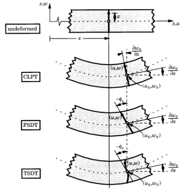
6.5 Classical Laminated Plate Theory (CLPT) ¶ The simplest of the ESL theories is the Classical Laminated Plate Theory (CLPT) which is an extension of the Classical Plate Theory to composite laminates Reddy, 2003 Reddy, 2003
Transverse normals remain straight after deformation;
Transverse normals do not experience elongation (ε z z = 0 \varepsilon_{zz} = 0 ε zz = 0
The transverse normals rotate so that they remain perpendicular to the mid-surface after deformation (no transverse shear takes place, i.e. γ y z = γ x z = 0 \gamma_{yz} = \gamma_{xz} = 0 γ yz = γ x z = 0 ϕ x = − ∂ w ∂ x \phi_x = -\frac{\partial w}{\partial x} ϕ x = − ∂ x ∂ w Figure 7
Figure 7: CLPT kinematics Castro, 2015
The displacement field using the CLPT Castro, 2015 (5)
u ( x , y , z ) = u 0 ( x , y ) − z w , x ( x , y ) v ( x , y , z ) = v 0 ( x , y ) − z w , y ( x , y ) w ( x , y , z ) = w 0 ( x , y ) \begin{split}
u(x, y, z) = u_0(x, y) - z w_{,x}(x, y) \\
v(x, y, z) = v_0(x, y) - z w_{,y}(x, y) \\
w(x, y, z) = w_0(x, y)
\end{split} u ( x , y , z ) = u 0 ( x , y ) − z w , x ( x , y ) v ( x , y , z ) = v 0 ( x , y ) − z w , y ( x , y ) w ( x , y , z ) = w 0 ( x , y ) For convenience, it is customary to omit the subscript “0” from the mid-surface displacements, which should be clear from the context.
6.6 First-order Shear Deformation Theory (FSDT) ¶ Also known as Reissner-Mindlin theory, the FSDT is the vastly most used ESL theory within finite element codes. Its popularity comes from fact that the rotations being decoupled from the deflections, enabling straightforward and compatible linear interpolation of displacements and rotations within different finite element formulations. The main kinematic features of the FSDT are:
Rotations disconnected from normal displacements ϕ x ( x , y ) ≠ − w , x ( x , y ) \phi_x(x, y) \neq -w_{,x} (x, y) ϕ x ( x , y ) = − w , x ( x , y )
Transverse normals do not experience elongation (ε z z = 0 \varepsilon_{zz} = 0 ε zz = 0
Transverse shear strains γ x z \gamma_{xz} γ x z γ y z \gamma_{yz} γ yz z z z shear correction factors are needed .
Figure 8: FSDT kinematics Castro, 2015
The displacement field using the FSDT Castro, 2015 (6)
u ( x , y , z ) = u 0 ( x , y ) + z ϕ x ( x , y ) v ( x , y , z ) = v 0 ( x , y ) + z ϕ y ( x , y ) w ( x , y , z ) = w ( x , y ) \begin{split}
u(x, y, z) = u_0(x, y) + z \phi_x(x, y) \\
v(x, y, z) = v_0(x, y) + z \phi_y(x, y) \\
w(x, y, z) = w(x, y)
\end{split} u ( x , y , z ) = u 0 ( x , y ) + z ϕ x ( x , y ) v ( x , y , z ) = v 0 ( x , y ) + z ϕ y ( x , y ) w ( x , y , z ) = w ( x , y ) Again, for convenience, it is customary to omit the subscript “0” from the mid-surface displacements, which should be clear from the context. Figure 9 Castro, 2015
Figure 9: Kinematic comparison between CLPT and FSDT Castro, 2015
Reddy proposed a third-order shear deformation theory that results in a second-order interpolation of the transverse shear strains Reddy, 2003, Chap. 11
Rotations disconnected from normal displacements ϕ x ( x , y ) ≠ − w , x ( x , y ) \phi_x(x, y) \neq -w_{,x} (x, y) ϕ x ( x , y ) = − w , x ( x , y )
Transverse normals do not experience elongation (ε z z = 0 \varepsilon_{zz} = 0 ε zz = 0
Consistent transverse shear strains γ x z ( x , y , z ) \gamma_{xz}(x, y, z) γ x z ( x , y , z ) γ y z ( x , y , z ) \gamma_{yz}(x, y, z) γ yz ( x , y , z ) shear correction factors are not needed .
A general third-order shear deformation theory would have 9 unknown field variables, as shown below:
u ( x , y , z ) = u 0 ( x , y ) + z ϕ x ( x , y ) + z 2 θ x ( x , y ) + z 3 λ x ( x , y ) v ( x , y , z ) = v 0 ( x , y ) + z ϕ y ( x , y ) + z 2 θ y ( x , y ) + z 3 λ y ( x , y ) w ( x , y , z ) = w 0 ( x , y ) \begin{split}
u(x, y, z) = u_0(x, y) + z \phi_x(x, y) + z^2 \theta_x(x, y) + z^3 \lambda_x(x, y) \\
v(x, y, z) = v_0(x, y) + z \phi_y(x, y) + z^2 \theta_y(x, y) + z^3 \lambda_y(x, y) \\
w(x, y, z) = w_0(x, y)
\end{split} u ( x , y , z ) = u 0 ( x , y ) + z ϕ x ( x , y ) + z 2 θ x ( x , y ) + z 3 λ x ( x , y ) v ( x , y , z ) = v 0 ( x , y ) + z ϕ y ( x , y ) + z 2 θ y ( x , y ) + z 3 λ y ( x , y ) w ( x , y , z ) = w 0 ( x , y ) Reddy proposed, already in 1984, to impose 4 traction-free boundary conditions, on the bottom and top faces of the laminate:
τ x z ( x , y , ± h 2 ) = 0 τ y z ( x , y , ± h 2 ) = 0 \tau_{xz}\left(x, y, \pm \frac{h}{2}\right) = 0 \qquad \tau_{yz}\left(x, y, \pm \frac{h}{2}\right) = 0 τ x z ( x , y , ± 2 h ) = 0 τ yz ( x , y , ± 2 h ) = 0 which then result in the following kinematic relation with 5 unknown field variables:
u ( x , y , z ) = u 0 ( x , y ) + z ϕ x ( x , y ) − 4 3 h 2 z 3 ( ϕ x ( x , y ) + w , x ( x , y ) ) v ( x , y , z ) = v 0 ( x , y ) + z ϕ y ( x , y ) − 4 3 h 2 z 3 ( ϕ y ( x , y ) + w , y ( x , y ) ) w ( x , y , z ) = w ( x , y ) \begin{split}
u(x, y, z) = u_0(x, y) + z \phi_x(x, y) - \frac{4}{3h^2} z^3 \big(\phi_x(x, y) + w_{,x}(x, y)\big) \\
v(x, y, z) = v_0(x, y) + z \phi_y(x, y) - \frac{4}{3h^2} z^3 \big(\phi_y(x, y) + w_{,y}(x, y)\big) \\
w(x, y, z) = w(x, y)
\end{split} u ( x , y , z ) = u 0 ( x , y ) + z ϕ x ( x , y ) − 3 h 2 4 z 3 ( ϕ x ( x , y ) + w , x ( x , y ) ) v ( x , y , z ) = v 0 ( x , y ) + z ϕ y ( x , y ) − 3 h 2 4 z 3 ( ϕ y ( x , y ) + w , y ( x , y ) ) w ( x , y , z ) = w ( x , y ) Again, for convenience, it is customary to omit the subscript “0” from the mid-surface displacements, which should be clear from the context. Figure 10 Reddy, 2003
Figure 10: Kinematic comparison between CLPT, FSDT and TSDT Reddy, 2003
7 ESL equations for plates ¶ 7.1 CLPT for plates ¶ For a plate, the displacement field can be approximated using the CLPT using the definitions of Eq. (5) (1) Castro, 2015
ε x x = u , x − z w , x x + 1 2 ( ( z w , x x − u , x ) 2 + ( z w , x y − v , x ) 2 + w , x 2 ) ε y y = v , y − z w , y y + 1 2 ( ( z w , x y − u , y ) 2 + ( z w , y y − v , y ) 2 + w , y 2 ) ε z z = 0 (thickness remains constant during bending) γ x y = u , y + v , x − 2 z w , x y + ( z w , x x − u , x ) ( z w , x y − u , y ) + ( z w , x y − v , x ) ( z w , y y − v , y ) + w , x w , y γ x z = 0 γ y z = 0 \begin{split}
\varepsilon_{xx} = u_{,x} - z w_{,xx} + \frac{1}{2}\left((z w_{,xx} - u_{,x})^2 + (z w_{,xy} - v_{,x})^2 + w_{,x}^2\right) \\
\varepsilon_{yy} = v_{,y} - z w_{,yy} + \frac{1}{2}\left((z w_{,xy} - u_{,y})^2 + (z w_{,yy} - v_{,y})^2 + w_{,y}^2\right) \\
\varepsilon_{zz} = 0 \text{ (thickness remains constant during bending)} \\
\gamma_{xy} = u_{,y} + v_{,x} - 2z w_{,xy} + (z w_{,xx} - u_{,x})(z w_{,xy} - u_{,y}) + (z w_{,xy} - v_{,x})(z w_{,yy} - v_{,y}) + w_{,x}w_{,y} \\
\gamma_{xz} = 0 \\
\gamma_{yz} = 0
\end{split} ε xx = u , x − z w , xx + 2 1 ( ( z w , xx − u , x ) 2 + ( z w , x y − v , x ) 2 + w , x 2 ) ε yy = v , y − z w , yy + 2 1 ( ( z w , x y − u , y ) 2 + ( z w , yy − v , y ) 2 + w , y 2 ) ε zz = 0 (thickness remains constant during bending) γ x y = u , y + v , x − 2 z w , x y + ( z w , xx − u , x ) ( z w , x y − u , y ) + ( z w , x y − v , x ) ( z w , yy − v , y ) + w , x w , y γ x z = 0 γ yz = 0 Using van Kármán kinematics, many of the nonlinear terms are simplified Castro, 2015
ε x x = u , x − z w , x x + 1 2 w , x 2 ε y y = v , y − z w , y y + 1 2 w , y 2 ε z z = 0 (thickness remains constant during bending) γ x y = u , y + v , x − 2 z w , x y + w , x w , y γ x z = 0 γ y z = 0 \begin{split}
\varepsilon_{xx} = u_{,x} - z w_{,xx} + \frac{1}{2}w_{,x}^2 \\
\varepsilon_{yy} = v_{,y} - z w_{,yy} + \frac{1}{2}w_{,y}^2 \\
\varepsilon_{zz} = 0 \text{ (thickness remains constant during bending)} \\
\gamma_{xy} = u_{,y} + v_{,x} - 2z w_{,xy} + w_{,x}w_{,y} \\
\gamma_{xz} = 0 \\
\gamma_{yz} = 0
\end{split} ε xx = u , x − z w , xx + 2 1 w , x 2 ε yy = v , y − z w , yy + 2 1 w , y 2 ε zz = 0 (thickness remains constant during bending) γ x y = u , y + v , x − 2 z w , x y + w , x w , y γ x z = 0 γ yz = 0 7.2 FSDT for plates ¶ For a plate, the displacement field can be approximated using the FSDT using the definitions of Eq. (6) (1) Castro, 2015
ε x x = u , x + z ϕ x , x + 1 2 ( ( z ϕ x , x + u , x ) 2 + ( z ϕ y , x + v , x ) 2 + w , x 2 ) ε y y = v , y + z ϕ y , y + 1 2 ( ( z ϕ x , y + u , y ) 2 + ( z ϕ y , y + v , y ) 2 + w , y 2 ) ε z z = 0 (thickness remains constant during bending) γ x y = u , y + v , x + z ϕ x , y + z ϕ y , x + ( z ϕ x , x + u , x ) ( z ϕ x , y + u , y ) + ( z ϕ y , x + v , x ) ( z ϕ y , y + v , y ) + w , x w , y γ x z = ϕ x + w , x + ( z ϕ x , x + u , x ) ϕ x + ( z ϕ y , x + v , x ) ϕ y γ y z = ϕ y + w , y + ( z ϕ x , y + u , y ) ϕ x + ( z ϕ y , y + v , y ) ϕ y \begin{split}
\varepsilon_{xx} = u_{,x} + z \phi_{x,x} + \frac{1}{2}\left((z\phi_{x,x} + u_{,x})^2 + (z\phi_{y,x} + v_{,x})^2 + w_{,x}^2\right) \\
\varepsilon_{yy} = v_{,y} + z \phi_{y,y} + \frac{1}{2}\left((z\phi_{x,y} + u_{,y})^2 + (z\phi_{y,y} + v_{,y})^2 + w_{,y}^2\right) \\
\varepsilon_{zz} = 0 \text{ (thickness remains constant during bending)} \\
\gamma_{xy} = u_{,y} + v_{,x} + z\phi_{x,y} + z\phi_{y,x} + (z\phi_{x,x} + u_{,x})(z\phi_{x,y} + u_{,y}) + (z\phi_{y,x} + v_{,x})(z\phi_{y,y} + v_{,y}) + w_{,x}w_{,y} \\
\gamma_{xz} = \phi_x + w_{,x} + (z\phi_{x,x} + u_{,x})\phi_x + (z\phi_{y,x} + v_{,x})\phi_y \\
\gamma_{yz} = \phi_y + w_{,y} + (z\phi_{x,y} + u_{,y})\phi_x + (z\phi_{y,y} + v_{,y})\phi_y
\end{split} ε xx = u , x + z ϕ x , x + 2 1 ( ( z ϕ x , x + u , x ) 2 + ( z ϕ y , x + v , x ) 2 + w , x 2 ) ε yy = v , y + z ϕ y , y + 2 1 ( ( z ϕ x , y + u , y ) 2 + ( z ϕ y , y + v , y ) 2 + w , y 2 ) ε zz = 0 (thickness remains constant during bending) γ x y = u , y + v , x + z ϕ x , y + z ϕ y , x + ( z ϕ x , x + u , x ) ( z ϕ x , y + u , y ) + ( z ϕ y , x + v , x ) ( z ϕ y , y + v , y ) + w , x w , y γ x z = ϕ x + w , x + ( z ϕ x , x + u , x ) ϕ x + ( z ϕ y , x + v , x ) ϕ y γ yz = ϕ y + w , y + ( z ϕ x , y + u , y ) ϕ x + ( z ϕ y , y + v , y ) ϕ y Using van Kármán Kinematics:
ε x x = u , x + z ϕ x , x + 1 2 w , x 2 ε y y = v , y + z ϕ y , y + 1 2 w , y 2 ε z z = 0 (thickness remains constant during bending) γ x y = u , y + v , x + z ϕ x , y + z ϕ y , x + w , x w , y γ x z = ϕ x + w , x γ y z = ϕ y + w , y \begin{split}
\varepsilon_{xx} = u_{,x} + z \phi_{x,x} + \frac{1}{2}w_{,x}^2 \\
\varepsilon_{yy} = v_{,y} + z \phi_{y,y} + \frac{1}{2}w_{,y}^2 \\
\varepsilon_{zz} = 0 \text{ (thickness remains constant during bending)} \\
\gamma_{xy} = u_{,y} + v_{,x} + z\phi_{x,y} + z\phi_{y,x} + w_{,x}w_{,y} \\
\gamma_{xz} = \phi_x + w_{,x} \\
\gamma_{yz} = \phi_y + w_{,y}
\end{split} ε xx = u , x + z ϕ x , x + 2 1 w , x 2 ε yy = v , y + z ϕ y , y + 2 1 w , y 2 ε zz = 0 (thickness remains constant during bending) γ x y = u , y + v , x + z ϕ x , y + z ϕ y , x + w , x w , y γ x z = ϕ x + w , x γ yz = ϕ y + w , y It is usual to separate the terms multiplying “z” in the form of Eq. (12)
ε = { ε x x ε y y 2 ε x y } = { u 0 , x v 0 , y u 0 , y + v 0 , x } + z { ϕ x , x ϕ y , y ϕ x , y + ϕ y , x } γ = { 2 ε y z 2 ε x z } = { γ y z γ x z } = { w , y + ϕ y w , x + ϕ x } \begin{split}
\boldsymbol{\varepsilon} = \left\{ \begin{matrix} \varepsilon_{xx} \\ \varepsilon_{yy} \\ 2\varepsilon_{xy} \end{matrix} \right\} = \left\{ \begin{matrix} u_{0,x} \\ v_{0,y} \\ u_{0,y} + v_{0,x} \end{matrix} \right\} + z \left\{ \begin{matrix} \phi_{x,x} \\ \phi_{y,y} \\ \phi_{x,y} + \phi_{y,x} \end{matrix} \right\} \\
\boldsymbol{\gamma} = \left\{ \begin{matrix} 2\varepsilon_{yz} \\ 2\varepsilon_{xz} \end{matrix} \right\} = \left\{ \begin{matrix} \gamma_{yz} \\ \gamma_{xz} \end{matrix} \right\} = \left\{ \begin{matrix} w_{,y} + \phi_y \\ w_{,x} + \phi_x \end{matrix} \right\}
\end{split} ε = ⎩ ⎨ ⎧ ε xx ε yy 2 ε x y ⎭ ⎬ ⎫ = ⎩ ⎨ ⎧ u 0 , x v 0 , y u 0 , y + v 0 , x ⎭ ⎬ ⎫ + z ⎩ ⎨ ⎧ ϕ x , x ϕ y , y ϕ x , y + ϕ y , x ⎭ ⎬ ⎫ γ = { 2 ε yz 2 ε x z } = { γ yz γ x z } = { w , y + ϕ y w , x + ϕ x } or, using Voigt’s notation:
ε = ε ( 0 ) + z ε ( 1 ) γ = γ ( 0 ) \begin{split}
\boldsymbol{\varepsilon} = \boldsymbol{\varepsilon}^{(0)} + z\boldsymbol{\varepsilon}^{(1)} \\
\boldsymbol{\gamma} = \boldsymbol{\gamma}^{(0)}
\end{split} ε = ε ( 0 ) + z ε ( 1 ) γ = γ ( 0 ) Note that all relations presented for the FSDT represent a more general case than the CLPT, and can be directly converted to the latter by doing:
ϕ x = − w , x ϕ y = − w , y γ x z = 0 γ y z = 0 \begin{split}
\phi_x = -w_{,x} \\
\phi_y = -w_{,y} \\
\gamma_{xz} = 0 \\
\gamma_{yz} = 0
\end{split} ϕ x = − w , x ϕ y = − w , y γ x z = 0 γ yz = 0 7.3 TSDT for plates ¶ For a plate, the displacement field can be approximated using the TSDT using the definitions of Eq. (7) (1) Castro, 2025 (13)
ε x x = u , x + 1 2 w , x 2 + z ϕ x , x + z 3 ( − 4 3 h 2 ) ( ϕ x , x + w , x x ) ε y y = v , y + 1 2 w , y 2 + z ϕ y , y + z 3 ( − 4 3 h 2 ) ( ϕ y , y + w , y y ) γ x y = u , y + v , x + w , x w , y + z ϕ x , y + z ϕ y , x + z 3 ( − 4 3 h 2 ) ( ϕ x , y + ϕ y , x + 2 w , x y ) γ x z = ϕ x + w , x + z 2 ( − 4 h 2 ) ( ϕ x + w , x ) γ y z = ϕ y + w , y + z 2 ( − 4 h 2 ) ( ϕ y + w , y ) \begin{split}
\varepsilon_{xx} = u_{,x} + \frac{1}{2} w_{,x}^2 + z\phi_{x,x} + z^3 \left(-\frac{4}{3h^2}\right) (\phi_{x,x} + w_{,xx}) \\
\varepsilon_{yy} = v_{,y} + \frac{1}{2} w_{,y}^2 + z\phi_{y,y} + z^3 \left(-\frac{4}{3h^2}\right) (\phi_{y,y} + w_{,yy}) \\
\gamma_{xy} = u_{,y} + v_{,x} + w_{,x}w_{,y} + z\phi_{x,y} + z\phi_{y,x} + z^3 \left(-\frac{4}{3h^2}\right) (\phi_{x,y} + \phi_{y,x} + 2w_{,xy}) \\
\gamma_{xz} = \phi_x + w_{,x} + z^2 \left(-\frac{4}{h^2}\right) (\phi_x + w_{,x}) \\
\gamma_{yz} = \phi_y + w_{,y} + z^2 \left(-\frac{4}{h^2}\right) (\phi_y + w_{,y})
\end{split} ε xx = u , x + 2 1 w , x 2 + z ϕ x , x + z 3 ( − 3 h 2 4 ) ( ϕ x , x + w , xx ) ε yy = v , y + 2 1 w , y 2 + z ϕ y , y + z 3 ( − 3 h 2 4 ) ( ϕ y , y + w , yy ) γ x y = u , y + v , x + w , x w , y + z ϕ x , y + z ϕ y , x + z 3 ( − 3 h 2 4 ) ( ϕ x , y + ϕ y , x + 2 w , x y ) γ x z = ϕ x + w , x + z 2 ( − h 2 4 ) ( ϕ x + w , x ) γ yz = ϕ y + w , y + z 2 ( − h 2 4 ) ( ϕ y + w , y ) or, using Voigt’s notation:
ε = { ε x x ε y y 2 ε x y } = { u 0 , x v 0 , y u 0 , y + v 0 , x } + z { ϕ x , x ϕ y , y ϕ x , y + ϕ y , x } + z 3 ( − 4 3 h 2 ) { ϕ x , x + w , x x ϕ y , y + w , y y ϕ x , y + ϕ y , x + 2 w , x y } γ = { 2 ε y z 2 ε x z } = { γ y z γ x z } = { w , y + ϕ y w , x + ϕ x } + z 2 ( − 4 h 2 ) { w , y + ϕ y w , x + ϕ x } \begin{split}
\boldsymbol{\varepsilon} = \left\{ \begin{matrix} \varepsilon_{xx} \\ \varepsilon_{yy} \\ 2\varepsilon_{xy} \end{matrix} \right\} = \left\{ \begin{matrix} u_{0,x} \\ v_{0,y} \\ u_{0,y} + v_{0,x} \end{matrix} \right\} + z \left\{ \begin{matrix} \phi_{x,x} \\ \phi_{y,y} \\ \phi_{x,y} + \phi_{y,x} \end{matrix} \right\} + z^3 \left(-\frac{4}{3h^2}\right) \left\{ \begin{matrix} \phi_{x,x} + w_{,xx} \\ \phi_{y,y} + w_{,yy} \\ \phi_{x,y} + \phi_{y,x} + 2w_{,xy} \end{matrix} \right\} \\
\boldsymbol{\gamma} = \left\{ \begin{matrix} 2\varepsilon_{yz} \\ 2\varepsilon_{xz} \end{matrix} \right\} = \left\{ \begin{matrix} \gamma_{yz} \\ \gamma_{xz} \end{matrix} \right\} = \left\{ \begin{matrix} w_{,y} + \phi_y \\ w_{,x} + \phi_x \end{matrix} \right\} + z^2 \left(-\frac{4}{h^2}\right) \left\{ \begin{matrix} w_{,y} + \phi_y \\ w_{,x} + \phi_x \end{matrix} \right\}
\end{split} ε = ⎩ ⎨ ⎧ ε xx ε yy 2 ε x y ⎭ ⎬ ⎫ = ⎩ ⎨ ⎧ u 0 , x v 0 , y u 0 , y + v 0 , x ⎭ ⎬ ⎫ + z ⎩ ⎨ ⎧ ϕ x , x ϕ y , y ϕ x , y + ϕ y , x ⎭ ⎬ ⎫ + z 3 ( − 3 h 2 4 ) ⎩ ⎨ ⎧ ϕ x , x + w , xx ϕ y , y + w , yy ϕ x , y + ϕ y , x + 2 w , x y ⎭ ⎬ ⎫ γ = { 2 ε yz 2 ε x z } = { γ yz γ x z } = { w , y + ϕ y w , x + ϕ x } + z 2 ( − h 2 4 ) { w , y + ϕ y w , x + ϕ x } which becomes:
ε = ε ( 0 ) + z ε ( 1 ) + z 3 ε ( 3 ) γ = γ ( 0 ) + z 2 γ ( 2 ) \begin{split}
\boldsymbol{\varepsilon} = \boldsymbol{\varepsilon}^{(0)} + z\boldsymbol{\varepsilon}^{(1)} + z^3\boldsymbol{\varepsilon}^{(3)} \\
\boldsymbol{\gamma} = \boldsymbol{\gamma}^{(0)} + z^2\boldsymbol{\gamma}^{(2)}
\end{split} ε = ε ( 0 ) + z ε ( 1 ) + z 3 ε ( 3 ) γ = γ ( 0 ) + z 2 γ ( 2 ) Again, the subscript “0” for the mid-surface expressions is usually omitted.
Castro, S. G. P. (2015). Semi-analytical tools for the analysis of laminated composite cylindrical and conical imperfect shells under various loading and boundary conditinos [Phdthesis, Technische Universität Clausthal]. 10.21268/20150210-154320 Castro, S. G. P. (2025). Stability of Structures: Kinematics, Equivalent Single-Layer Theories, and Energy-based Semi-Analytical Methods . 10.5281/zenodo.18957062 Castro, S. G. P., Mittelstedt, C., Monteiro, F. A. C., Arbelo, M. A., Ziegmann, G., & Degenhardt, R. (2014). Linear buckling predictions of unstiffened laminated composite cylinders and cones under various loading and boundary conditions using semi-analytical models. Composite Structures , 118 , 303–315. 10.1016/j.compstruct.2014.07.037 Castro, S. G. P., Mittelstedt, C., Monteiro, F. A. C., Arbelo, M. A., Degenhardt, R., & Ziegmann, G. (2015). A semi-analytical approach for linear and non-linear analysis of unstiffened laminated composite cylinders and cones under axial, torsion and pressure loads. Thin-Walled Structures , 90 , 61–73. 10.1016/j.tws.2015.01.002 Castro, S. G. P., Mittelstedt, C., Monteiro, F. A. C., Degenhardt, R., & Ziegmann, G. (2015). Evaluation of non-linear buckling loads of geometrically imperfect composite cylinders and cones with the Ritz method. Composite Structures , 122 , 284–299. 10.1016/j.compstruct.2014.11.050 Reddy, J. N. (2003). Mechanics of Laminated Composite Plates and Shells . CRC Press. 10.1201/b12409