Basic principles

This first chapter presents the basic principles used to produce the system of equations to be solved.

1Principle of minimum potential energy¶

The total potential energy $V$ can be decomposed into elastic energy $U$, and the work due to external forces $W_{ext}$:

This potential becomes stationary when:

1.1Strain Energy¶

The general expression for the strain energy when $\boldsymbol{\sigma}$ increases linearly with $\boldsymbol{epsilon}$ is:

The variation of this expression, valid also for the case of $\boldsymbol{\sigma}$ being a non-linear function of $\boldsymbol{\varepsilon}$, renders:

To calculate the strain energy in semi-analytical formulations of plates and shells, it is convenient to represent the second-order tensors of strain and stress are represented as vectors, according to Voigt’s notation Voigt, 1910.

Given the 3D stress state of a material point illustrated in Figure 1, the components of the stress tensor $\sigma_{ij}$ can be aligned in a vector as in Eq. (1).

where:

• $\sigma_{11}$ - Normal in $x_1$

• $\sigma_{22}$ - Normal in $x_2$

• $\sigma_{33}$ - Normal in $x_3$ (thickness direction)

• $\tau_{23}$ - Transverse shear 23

• $\tau_{13}$ - Transverse shear 13

• $\tau_{12}$ - In-plane shear 12

A general constitutive relation for semi-analytical models, which show stresses relate to strains, can be written based on Voigt’s notation:

where $\boldsymbol{C}$ is the constitutive matrix.

Not all stress components shown in Eq. are relevant when calculating thin-walled structures. For plane stress using the Classical Laminated Plate Theory (CLPT):

For plane stress using the First- or Third-order Shear Deformation Theory (FSDT or TSDT):

The strains are usually expressed in terms of displacements in the so called kinematic equations, which can be generally written using Voigt’s notation as:

where $\boldsymbol{B} \equiv$ differentiation operator matrix, $\boldsymbol{u}(x,y,z) \equiv$ continuous displacement field.

1.1.1Finite elements¶

In finite elemets, interpolation functions are used to approximate the displacement field within each finite element, which can be generally written as:

where $\boldsymbol{\bar{u}} \equiv$ nodal displacements and $\boldsymbol{S}(x,y,z) \equiv$ interpolation (shape) functions valid only within the domain of one finite element.

Example for quadrilateral elements:

From the kinematic equations: $\boldsymbol{\varepsilon} = \boldsymbol{B}\boldsymbol{u}$, the differentiation operator $\boldsymbol{B}$ will contain the proper derivatives of the interpolation functions corresponding to a given finite element.

The stress strain relation $\boldsymbol{\sigma} = \boldsymbol{C}\boldsymbol{\varepsilon}$ will highly depend on each case. For trusses and beam (uniaxial stress), it can be simply $\sigma_{xx} = E\varepsilon_{xx}$, for plates this becomes more complicated, as covered later.

In finite elements, the strain energy can be thus expressed as:

Replacing $\boldsymbol{\sigma} = \boldsymbol{C}\boldsymbol{\varepsilon}$, for $\boldsymbol{C} = \boldsymbol{C}^\top$:

Replacing and $\boldsymbol{\varepsilon} = \boldsymbol{B}\boldsymbol{\bar{u}}$:

where $\boldsymbol{K}$ is the constitutive stiffness matrix, usually referred to as simply the stiffness matrix:

For finite elements, the rows and columns of $\boldsymbol{K}$ correspond to the degrees-of-freedom built by the assembly of all finite elements. The integration over the 3-dimensional domain $\Omega$ is performed in a piece-wise manner within the domain of each finite element $\Omega_e$.

The integration of $\boldsymbol{K}_e$ can be efficiently done numerically due to the local support of the integration points (only affect the stiffness of the corresponding element).

1.1.2Energy-based semi-analytical methods¶

In energy-based methods, such as the well-known Ritz method, the shape functions are expressed in terms of continuous functions instead of nodal degrees-of-freedom:

where $\boldsymbol{\bar{c}} \equiv$ amplitude of each term of the shape functions, $\boldsymbol{S}(x,y,z) \equiv$ shape functions valid within the entire domain of the semi-analytical model, which can be an entire plate, an entire shell, or parts of a structure in the case of multi-domain semi-analytical models.

Example for deflection of simply supported plate $\xi = x/a$, $\eta = y/b$:

From the kinematic equations: $\boldsymbol{\varepsilon} = \boldsymbol{B}\boldsymbol{u}$, the differentiation operator $\boldsymbol{B}$ will contain the proper derivatives of the shape functions.

The strain energy for the Ritz method can thus be expressed as:

Replacing $\boldsymbol{\sigma} = \boldsymbol{C}\boldsymbol{\varepsilon}$, for $\boldsymbol{C} = \boldsymbol{C}^\top$:

Replacing and $\boldsymbol{\varepsilon} = \boldsymbol{B}\boldsymbol{c}$:

with the constitutive stiffness matrix defined as:

In the Ritz Method, the rows and columns of $\boldsymbol{K}$ correspond to the degrees-of-freedom that depend on the number of function terms used in the displacement approximation. In single-domain semi-analytical models, there is only one integration domain $\Omega$, and the integration is usually performed analytically leading to very efficient methods that can analytically calculate the stiffness matrix, even for complex problems such as described by Castro et al. addressing the buckling of conical shells under combined load cases Castro et al., 2014. However, when numerical integration is needed, for instance due to variable stiffness or in non-linear analyses Castro et al., 2015, the non-local support of the integration can create a large disadvantage of the Ritz method when compared to the finite element. The non-local support comes from the fact that the approximation functions represent the whole domain, and each integration point requires the evaluation of the entire stiffness matrix because all degress-of-freedom are components of continuous functions that affect that integration point.

Therefore, one must be careful while implementing semi-analytical methods for cases of variable stiffness or non-linear analyses. The use of hierarchical polynomials as approximation functions enable such efficient implementations, because they allow the use of Gauss quadrature rules to efficiently perform the numerical integration. When trigonometric approximation functions are used the stiffness matrix can be integrated using the trapezoidal (piece-wise linear) or Simpson’s rule (piece-wise quadratic) Castro et al., 2015

1.2Work due to external forces¶

When considering tranction stresses $\boldsymbol{\bar{\sigma}}$ acting on the boundaries of the domain $\delta\Omega$, and body forces $\boldsymbol{b}$ acting on the entire volume of the domain $\Omega$, the following general expression for the work of external forces can be used:

The first variation of work due to external forces becomes:

where $\boldsymbol{F} \equiv$ external force vector, including body ($\boldsymbol{b}$) and boundary forces ($\boldsymbol{\bar{\sigma}}$).

1.3Semi-analytical static solution¶

Back to the stationary total potential energy functional:

The state of $V$ depends on a nodal displacement vector $\boldsymbol{\bar{u}}$ in the case of displacement-based finite elements. In the Ritz method, we can make $\boldsymbol{\bar{c}} = \boldsymbol{\bar{u}}$ such that $\boldsymbol{\bar{u}}$ represents the Ritz coefficients $\boldsymbol{\bar{c}}$ that contain the amplitude of each term of the shape functions.

We can represent $\delta V$ using Fréchet’s derivatives. In the case of linear analyses:

Thus, $V' = \boldsymbol{R}$, or a residual force vector, with $V'$ being the first Fréchet’s derivative of $V$. Using the definition for the total potential energy, the first variation becomes:

2Approximation functions¶

The orthogonal trigonometric series is the simplest solution for Eq. (1).

However, when a general set of boundary conditions is needed, or whenever a skewed buckling mode is possible, a more robust approximation for the displacement field is required. Castro and Donadon Castro & Donadon, 2017 present Rodrigues’ form of Legendre hierarchic orthogonal polynomials Peano, 1976De-Chao, 1986, largely applied by Bardell et al. on the vibration problems Bardell, 1991Bardell et al., 1997Bardell et al., 1997. In this form the first four terms $i = 1,2,3,4$ consist of Hermite cubic polynomials:

with $\chi \in \{\xi, \eta, \zeta\}$, and for any $i > 4$:

where $q!! = q(q - 2) \dots (2 \text{ or } 1)$ such that $0!! = 1$, and $(i/2)$ in the summation is an integer division. The binary flags $\delta_{t1}$, $\delta_{r1}$, $\delta_{t2}$ and $\delta_{r2}$ are equal to 0 or 1, and used in the first four terms of Rodrigues polynomials to enable or disable the translation and rotation of each domain boundary, as illustrated in Figure 2. From the fifth term onwards, the translation and rotation at the boundaries are always zero, such that they are use to increase the interpolation order in the inner part of the domain, as illustrated in Figure 3. Flag $\delta_{t1}$ is used to control the translation at boundary ($\chi = -1$), which is possible because using Rodrigues polynomials this is the only term among all terms in the approximation function that produces $P_i(\chi = -1) = 1$. Similarly, $\delta_{t2}$ is used to control the translation at boundary 2 ($\chi = +1$). The rotation at $\chi = -1$ and $\chi = +1$ is respectively controlled using $\delta_{r1}$ and $\delta_{r2}$, since they are the only terms that produce a non-null rotation $\partial P / \partial \chi$ at each respective domain boundary. The use of rotation is specially important in FSDT or TSDT formulations. Vescovini et al. Vescovini et al., 2018 investigated the sparsity of the systems produced by different shape functions, positively supporting the use of these Legendre hierarchical polynomials.

Take the plate-like domain shown in Figure 4. A general expression for the 3D displacement field is:

using Legendre polynomials and a summation convention for repeated indices:

with $1 \le [i,j,k] \le n_{[x,y,z]}$ where $n_[x,y,z]$ represents the number of terms in each global coordinate direction. The natural coordinates $\xi$, $\eta$ and $\zeta$ are defined as follows for a plate:

For the sake of completeness, let’s also write the expressions for the displacement field using explicit summation:

and using vector notation:

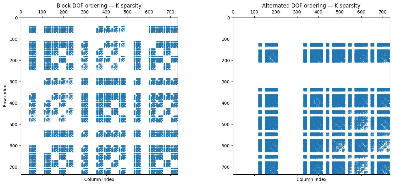
where $\boldsymbol{c}$ contains all coefficients $c_{ijk}$ for $1 \le [i,j,k] \le n_{[x,y,z]}$. The sequence in which the coefficients are placed is arbritrary and does not affect the level of sparsity of the stiffness matrix or other structural matrices, but it does affect the bandwidth of these matrices, which significantly affects the overall efficiency and numerically stability of the implementation. To illustrate the differences in defree-of-freedom (DOF) ordering, a practical example of the buckling of a plate using 3D elasticity is investigated in depth in this notebook. There, the DOF are stored in a block- and alternated-based approach. The results are compared in detail, and the sparsity of the stiffness matrix$~\boldsymbol{K}$ is illustrated in Figure 5. A detailed formulation of this problem is provided in details in Section 2.

3Neutral Equilibrium Criterion¶

The neutral equilibrium of a vertical slender beam is illustrated in Figure 6

Given the expression for $V'$:

The second variation of $V$ becomes:

In a system without follower forces $\delta \boldsymbol{\hat{\sigma}} = \delta \boldsymbol{\hat{b}} = \boldsymbol{0}$, and we can consider $\delta^2 \boldsymbol{u} \ll \delta \boldsymbol{u}$:

The first integral represents the nonlinear constitutive stiffness, whereas the second integral represents the geometric stiffness matrix. If the strains can be represented as:

And the stresses as:

Then:

The neutral equilibrium criterion states that:

This term represents the constitutive stiffness matrix:

From a linear fundamental (pre-buckling) state we have that $\boldsymbol{B}_{NL} = \boldsymbol{0}$:

such that:

where $\boldsymbol{K}_G$ represents the geometric stiffness matrix. Note that this expression must be true for any variation $\delta \boldsymbol{\bar{u}}$, such that $\boldsymbol{K}_0 + \lambda\boldsymbol{K}_G$ must be singular for the expression to be generaly true, hence:

where $\lambda$ is a load multiplier applied to the initial stress state defining $\boldsymbol{K}_G$. This is the well-known eigenvalue problem for buckling, also referred to as linear buckling equation.