Practice, block vs. alternated degree-of-freedom ordering in 3D plate buckling¶

This notebook compares two strategies for positioning the degrees of freedom (DOFs) inside the global stiffness matrix $\mathbf{K}$ and geometric stiffness matrix $\mathbf{K}_G$ of a 3D plate buckling problem solved with the Ritz method using Legendre polynomial bases.

Both formulations solve the same physical problem — the only difference is the order in which the $u$ , $v$ , $w$ coefficients are stored in the global DOF vector $\mathbf{q}$ .

Strategy	Global DOF vector layout	Index of $u_n$	Index of $v_n$	Index of $w_n$
Block	$[u_1 \cdots u_M \mid v_1 \cdots v_M \mid w_1 \cdots w_M]$	$n$	$M + n$	$2M + n$
Alternated	$[u_1, v_1, w_1, \; u_2, v_2, w_2, \; \cdots]$	$3n$	$3n + 1$	$3n + 2$

where $M = m_1 \times m_2 \times m_3$ is the number of basis function triplets.

The two orderings are related by a permutation matrix $\mathbf{P}$ such that $\mathbf{q}_\text{alt} = \mathbf{P}\,\mathbf{q}_\text{block}$ , and consequently:

\mathbf{K}_\text{alt} = \mathbf{P}\,\mathbf{K}_\text{block}\,\mathbf{P}^T, \qquad \mathbf{K}_{G,\text{alt}} = \mathbf{P}\,\mathbf{K}_{G,\text{block}}\,\mathbf{P}^T

Since the eigenvalues of a generalized eigenvalue problem are invariant under simultaneous congruence transformation, both orderings must produce identical eigenvalues. This notebook verifies that claim and examines how DOF ordering affects sparsity patterns and solver behavior.

1Install required libraries¶

!python -m pip install buckling structsolve > tmp.txt

2Import required libraries¶

import numpy as np
import matplotlib.pyplot as plt
import plotly.graph_objects as go
from scipy.special import roots_legendre
from scipy.sparse import csc_matrix
from structsolve import lb

from buckling.legendre import vecf, vecfxi

3Approximation space and quadrature¶

We define the polynomial expansion orders ( $m_1, m_2, m_3$ ) for the displacement field $(u, v, w)$ along the $x, y, z$ axes. The total degrees of freedom is $N = 3 \times m_1 \times m_2 \times m_3$ , and the number of basis function triplets is $M = m_1 \times m_2 \times m_3$ .

Integration points and weights are computed using Gauss-Legendre quadrature. The number of integration points ( $2m - 1$ ) is chosen to exactly integrate the stiffness terms formulated by the polynomial bases.

m1 = m2 = 7
m3 = 5
M = m1 * m2 * m3       # DOFs per displacement component
N = 3 * M              # Total DOFs

print(f'm1 = {m1}, m2 = {m2}, m3 = {m3}')
print(f'DOFs per component (M) = {M}')
print(f'Total DOF (N) = {N}')

pts1, weights1 = roots_legendre(2*m1 - 1)
pts2, weights2 = roots_legendre(2*m2 - 1)
pts3, weights3 = roots_legendre(2*m3 - 1)

m1 = 7, m2 = 7, m3 = 5
DOFs per component (M) = 245
Total DOF (N) = 735

4Material, geometry, and boundary conditions¶

Isotropic material properties and plate dimensions are defined. A fundamental compressive pre-stress state (sigxx = -1.0) is applied to evaluate the geometric stiffness.

Boundary constraints (xit1, xir1, etc.) are defined to enforce essential boundary conditions directly on the trial functions.

E = 200.0e9
nu = 0.3
G = E / (2 * (1 + nu))

a = 0.3
b = 0.1
h = 0.003

sigxx = -1.0

xit1, xir1 = 0, 1
xit2, xir2 = 0, 1
etat1, etar1 = 0, 1
etat2, etar2 = 0, 1
zetat1, zetar1 = 1, 1
zetat2, zetar2 = 1, 1

5Pre-allocation and helper functions¶

Both DOF orderings share the same set of shape-function vectors ( $S_u, S_v, S_w$ and their spatial derivatives), stiffness matrices $\mathbf{K}$ and $\mathbf{K}_G$ , and the same in-place outer-product helper addouter.

The only difference between the two approaches is where each coefficient is placed within these length- $N$ vectors — the physics (strain definitions, constitutive law, Jacobian) is identical.

def make_arrays():
    """Allocate fresh working arrays for one assembly pass."""
    Su  = np.zeros(N); Sv  = np.zeros(N); Sw  = np.zeros(N)
    Sux = np.zeros(N); Svx = np.zeros(N); Swx = np.zeros(N)
    Suy = np.zeros(N); Svy = np.zeros(N); Swy = np.zeros(N)
    Suz = np.zeros(N); Svz = np.zeros(N); Swz = np.zeros(N)
    buff = np.zeros((N, N))
    K  = np.zeros((N, N))
    KG = np.zeros((N, N))
    return (Su, Sv, Sw, Sux, Svx, Swx, Suy, Svy, Swy,
            Suz, Svz, Swz, buff, K, KG)

def addouter(matrix, vec1, vec2, buff):
    """In-place addition of outer product to a target matrix."""
    np.outer(vec1, vec2, out=buff)
    matrix += buff

5.1DOF ordering: block layout¶

In the block (sequential) ordering, all $u$ -coefficients come first, then all $v$ -coefficients, then all $w$ -coefficients:

\mathbf{q}_\text{block} = \bigl[\underbrace{u_1, u_2, \ldots, u_M}_{\text{indices } 0 \ldots M{-}1} \;\big|\; \underbrace{v_1, v_2, \ldots, v_M}_{\text{indices } M \ldots 2M{-}1} \;\big|\; \underbrace{w_1, w_2, \ldots, w_M}_{\text{indices } 2M \ldots 3M{-}1}\bigr]

In code, this maps to slice-based indexing:

Su[:M]       = flat   # u-component
Sv[M:2*M]    = flat   # v-component
Sw[2*M:]     = flat   # w-component

63D numerical integration — block DOF assembly¶

The linear stiffness matrix $\mathbf{K}$ and geometric stiffness matrix $\mathbf{K}_G$ are built via numerical integration over the 3D domain using the block DOF layout.

(Su, Sv, Sw, Sux, Svx, Swx, Suy, Svy, Swy,
 Suz, Svz, Swz, buff, K_block, KG_block) = make_arrays()

for xi, wxi in zip(pts1, weights1):
    P_xi = vecf(m1, xi, xit1, xir1, xit2, xir2)
    Px_xi = vecfxi(m1, xi, xit1, xir1, xit2, xir2)
    for eta, weta in zip(pts2, weights2):
        P_eta = vecf(m2, eta, etat1, etar1, etat2, etar2)
        Px_eta = vecfxi(m2, eta, etat1, etar1, etat2, etar2)
        for zeta, wzeta in zip(pts3, weights3):
            P_zeta = vecf(m3, zeta, zetat1, zetar1, zetat2, zetar2)
            Px_zeta = vecfxi(m3, zeta, zetat1, zetar1, zetat2, zetar2)
            weight = wxi * weta * wzeta

            # --- Block indexing: Su[:M], Sv[M:2M], Sw[2M:] ---
            Pi, Pj, Pk = np.meshgrid(P_xi, P_eta, P_zeta, indexing='ij')
            flat = (Pi*Pj*Pk).flatten()
            Su[:M] = flat;  Sv[M:2*M] = flat;  Sw[2*M:] = flat

            Pxi, Pj, Pk = np.meshgrid(Px_xi, P_eta, P_zeta, indexing='ij')
            flat_x = (Pxi*Pj*Pk*(2/a)).flatten()
            Sux[:M] = flat_x;  Svx[M:2*M] = flat_x;  Swx[2*M:] = flat_x

            Pi, Pxj, Pk = np.meshgrid(P_xi, Px_eta, P_zeta, indexing='ij')
            flat_y = (Pi*Pxj*Pk*(2/b)).flatten()
            Suy[:M] = flat_y;  Svy[M:2*M] = flat_y;  Swy[2*M:] = flat_y

            Pi, Pj, Pxk = np.meshgrid(P_xi, P_eta, Px_zeta, indexing='ij')
            flat_z = (Pi*Pj*Pxk*(2/h)).flatten()
            Suz[:M] = flat_z;  Svz[M:2*M] = flat_z;  Swz[2*M:] = flat_z

            NL = 0
            exx = Sux + NL*1/2*(Sux**2 + Svx**2 + Swx**2)
            eyy = Svy + NL*1/2*(Suy**2 + Svy**2 + Swy**2)
            ezz = Swz + NL*1/2*(Suz**2 + Svz**2 + Swz**2)
            gxy = Suy + Svx + NL*(Sux*Suy + Svx*Svy + Swx*Swy)
            gxz = Suz + Swx + NL*(Sux*Suz + Svx*Svz + Swx*Swz)
            gyz = Svz + Swy + NL*(Suy*Suz + Svy*Svz + Swy*Swz)

            C = E / ((1 - 2*nu)*(1 + nu))
            Sxx = C * ((1 - nu)*exx + nu*eyy + nu*ezz)
            Syy = C * (nu*exx + (1 - nu)*eyy + nu*ezz)
            Szz = C * (nu*exx + nu*eyy + (1 - nu)*ezz)
            Txy = G * gxy;  Txz = G * gxz;  Tyz = G * gyz

            detJ = a * b * h / 8

            addouter(K_block, detJ*weight*Sxx, exx, buff)
            addouter(K_block, detJ*weight*Syy, eyy, buff)
            addouter(K_block, detJ*weight*Szz, ezz, buff)
            addouter(K_block, detJ*weight*Txy, gxy, buff)
            addouter(K_block, detJ*weight*Txz, gxz, buff)
            addouter(K_block, detJ*weight*Tyz, gyz, buff)

            addouter(KG_block, detJ*weight*sigxx*Swx, Swx, buff)

print('Block assembly done.')

Block assembly done.

6.1Eigenvalue solution — block DOF¶

eigvals_block, eigvecs_block = lb(csc_matrix(K_block), csc_matrix(KG_block),
                                  sparse_solver=False)

eigvals_block_sparse, eigvecs_block_sparse = lb(csc_matrix(K_block), csc_matrix(KG_block),
                                  sparse_solver=True)

D = E * h**3 / (12 * (1 - nu**2))
lbd_block = eigvals_block[0] * sigxx * b**2 * h / np.pi**2 / D

print(f'Block ordering — normalized buckling load: {lbd_block:.6f}')
print(f'First 5 eigenvalues: {eigvals_block[:5]}')

Running linear buckling analysis...
		Eigenvalue solver... 
			Removing null columns...
				360 columns removed
			finished!
			eigh() solver...
			finished!
		finished!
	first 5 eigenvalues:
		1522040927.7001903
		2282698902.6239214
		7425108997.486525
		8109202084.400536
		14777273133.311518
Running linear buckling analysis...
		Eigenvalue solver... 
			eigsh() solver (sigma=1.0)...
				WARNING: Factor is exactly singular
			aborted!
			Removing null columns...
				360 columns removed
			finished!
			eigsh() solver (sigma=4.1489519909504436e-10)...
			finished!
		finished!
	first 5 eigenvalues:
		1522040927.6879106
		2282698902.658078
		7425108997.522677
		8109202084.386688
		14777273133.059479
Block ordering — normalized buckling load: -9.355709
First 5 eigenvalues: [1.52204093e+09 2.28269890e+09 7.42510900e+09 8.10920208e+09
 1.47772731e+10]

/opt/miniconda3/lib/python3.13/site-packages/structsolve/linear_buckling.py:93: RuntimeWarning: divide by zero encountered in divide
  eigvals = -1./eigvals
/opt/miniconda3/lib/python3.13/site-packages/structsolve/linear_buckling.py:12: MatrixRankWarning: Matrix is exactly singular
  y = spsolve(K, KG @ x)

7DOF ordering: alternated (interleaved) layout¶

In the alternated ordering, the three displacement components for each basis triplet $(i, j, k)$ are grouped together:

\mathbf{q}_\text{alt} = \bigl[u_1, v_1, w_1, \; u_2, v_2, w_2, \; \ldots, \; u_M, v_M, w_M\bigr]

The $n$ -th basis triplet maps to global indices $3n$ , $3n{+}1$ , $3n{+}2$ for $u$ , $v$ , $w$ respectively. In code, this maps to stride-based indexing:

Su[0::3] = flat   # u-component (every 3rd entry starting at 0)
Sv[1::3] = flat   # v-component (every 3rd entry starting at 1)
Sw[2::3] = flat   # w-component (every 3rd entry starting at 2)

This layout is common in finite-element codes where nodal DOFs are kept together for easier application of boundary conditions and contact constraints.

7.13D numerical integration — alternated DOF assembly¶

The identical triple Gauss-Legendre loop is executed, but the shape-function vectors are filled using the alternated (interleaved) index mapping. The physics (strain definitions, constitutive law, Jacobian) remain unchanged.

(Su, Sv, Sw, Sux, Svx, Swx, Suy, Svy, Swy,
 Suz, Svz, Swz, buff, K_alt, KG_alt) = make_arrays()

for xi, wxi in zip(pts1, weights1):
    P_xi = vecf(m1, xi, xit1, xir1, xit2, xir2)
    Px_xi = vecfxi(m1, xi, xit1, xir1, xit2, xir2)
    for eta, weta in zip(pts2, weights2):
        P_eta = vecf(m2, eta, etat1, etar1, etat2, etar2)
        Px_eta = vecfxi(m2, eta, etat1, etar1, etat2, etar2)
        for zeta, wzeta in zip(pts3, weights3):
            P_zeta = vecf(m3, zeta, zetat1, zetar1, zetat2, zetar2)
            Px_zeta = vecfxi(m3, zeta, zetat1, zetar1, zetat2, zetar2)
            weight = wxi * weta * wzeta

            # --- Alternated indexing: Su[0::3], Sv[1::3], Sw[2::3] ---
            Pi, Pj, Pk = np.meshgrid(P_xi, P_eta, P_zeta, indexing='ij')
            flat = (Pi*Pj*Pk).flatten()
            Su[0::3] = flat;  Sv[1::3] = flat;  Sw[2::3] = flat

            Pxi, Pj, Pk = np.meshgrid(Px_xi, P_eta, P_zeta, indexing='ij')
            flat_x = (Pxi*Pj*Pk*(2/a)).flatten()
            Sux[0::3] = flat_x;  Svx[1::3] = flat_x;  Swx[2::3] = flat_x

            Pi, Pxj, Pk = np.meshgrid(P_xi, Px_eta, P_zeta, indexing='ij')
            flat_y = (Pi*Pxj*Pk*(2/b)).flatten()
            Suy[0::3] = flat_y;  Svy[1::3] = flat_y;  Swy[2::3] = flat_y

            Pi, Pj, Pxk = np.meshgrid(P_xi, P_eta, Px_zeta, indexing='ij')
            flat_z = (Pi*Pj*Pxk*(2/h)).flatten()
            Suz[0::3] = flat_z;  Svz[1::3] = flat_z;  Swz[2::3] = flat_z

            NL = 0
            exx = Sux + NL*1/2*(Sux**2 + Svx**2 + Swx**2)
            eyy = Svy + NL*1/2*(Suy**2 + Svy**2 + Swy**2)
            ezz = Swz + NL*1/2*(Suz**2 + Svz**2 + Swz**2)
            gxy = Suy + Svx + NL*(Sux*Suy + Svx*Svy + Swx*Swy)
            gxz = Suz + Swx + NL*(Sux*Suz + Svx*Svz + Swx*Swz)
            gyz = Svz + Swy + NL*(Suy*Suz + Svy*Svz + Swy*Swz)

            C = E / ((1 - 2*nu)*(1 + nu))
            Sxx = C * ((1 - nu)*exx + nu*eyy + nu*ezz)
            Syy = C * (nu*exx + (1 - nu)*eyy + nu*ezz)
            Szz = C * (nu*exx + nu*eyy + (1 - nu)*ezz)
            Txy = G * gxy;  Txz = G * gxz;  Tyz = G * gyz

            detJ = a * b * h / 8

            addouter(K_alt, detJ*weight*Sxx, exx, buff)
            addouter(K_alt, detJ*weight*Syy, eyy, buff)
            addouter(K_alt, detJ*weight*Szz, ezz, buff)
            addouter(K_alt, detJ*weight*Txy, gxy, buff)
            addouter(K_alt, detJ*weight*Txz, gxz, buff)
            addouter(K_alt, detJ*weight*Tyz, gyz, buff)

            addouter(KG_alt, detJ*weight*sigxx*Swx, Swx, buff)

print('Alternated assembly done.')

Alternated assembly done.

7.2Eigenvalue solution — alternated DOF¶

eigvals_alt, eigvecs_alt = lb(csc_matrix(K_alt), csc_matrix(KG_alt),
                              sparse_solver=False)

eigvals_alt_sparse, eigvecs_alt_sparse = lb(csc_matrix(K_alt), csc_matrix(KG_alt),
                              sparse_solver=True)

lbd_alt = eigvals_alt[0] * sigxx * b**2 * h / np.pi**2 / D

print(f'Alternated ordering — normalized buckling load: {lbd_alt:.6f}')
print(f'First 5 eigenvalues: {eigvals_alt[:5]}')

Running linear buckling analysis...
		Eigenvalue solver... 
			Removing null columns...
				360 columns removed
			finished!
			eigh() solver...
			finished!
		finished!
	first 5 eigenvalues:
		1522040927.695189
		2282698902.708363
		7425108997.673563
		8109202084.373646
		14777273133.24723
Running linear buckling analysis...
		Eigenvalue solver... 
			eigsh() solver (sigma=1.0)...
				WARNING: Factor is exactly singular
			aborted!
			Removing null columns...
				360 columns removed
			finished!
			eigsh() solver (sigma=3.018426128182952e-10)...
			finished!
		finished!
	first 5 eigenvalues:
		1522040927.6726487
		2282698902.651802
		7425108997.464223
		8109202084.340463
		14777273133.24027
Alternated ordering — normalized buckling load: -9.355709
First 5 eigenvalues: [1.52204093e+09 2.28269890e+09 7.42510900e+09 8.10920208e+09
 1.47772731e+10]

8Permutation equivalence verification¶

We now verify that $\mathbf{K}_\text{alt}$ and $\mathbf{K}_\text{block}$ are related by the permutation $\mathbf{P}$ that maps block indices to alternated indices:

P(n) = 3n, \quad P(M + n) = 3n + 1, \quad P(2M + n) = 3n + 2 \quad \text{for } n = 0, \ldots, M{-}1

If the two systems are truly equivalent, then $\mathbf{K}_\text{block}[\mathbf{P}^{-1}, \mathbf{P}^{-1}] = \mathbf{K}_\text{alt}$ element-wise.

# Build the permutation: perm[block_index] = alternated_index
perm = np.zeros(N, dtype=int)
for n in range(M):
    perm[n]       = 3*n       # u_n
    perm[M + n]   = 3*n + 1   # v_n
    perm[2*M + n] = 3*n + 2   # w_n

inv_perm = np.argsort(perm)
K_permuted  = K_block[np.ix_(inv_perm, inv_perm)]
KG_permuted = KG_block[np.ix_(inv_perm, inv_perm)]

print(f'max|K_permuted  - K_alt|  = {np.max(np.abs(K_permuted - K_alt)):.2e}')
print(f'max|KG_permuted - KG_alt| = {np.max(np.abs(KG_permuted - KG_alt)):.2e}')
print()
print('The matrices are identical under permutation => mathematically equivalent systems.')

max|K_permuted  - K_alt|  = 0.00e+00
max|KG_permuted - KG_alt| = 0.00e+00

The matrices are identical under permutation => mathematically equivalent systems.

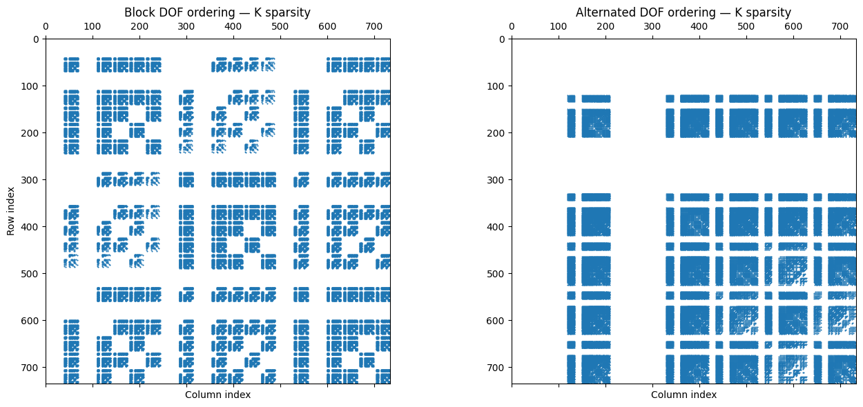
9Comparison of stiffness matrix sparsity patterns¶

Although the two systems have the same eigenvalues, their sparsity patterns differ dramatically. The block ordering produces a characteristic $3 \times 3$ block structure with three dense diagonal blocks ( $\mathbf{K}_{uu}$ , $\mathbf{K}_{vv}$ , $\mathbf{K}_{ww}$ ) and off-diagonal coupling blocks. The alternated ordering distributes the non-zeros more uniformly, producing a banded or semi-banded pattern.

These structural differences affect:

Memory layout: block ordering is more cache-friendly during assembly since consecutive DOFs often share the same basis function type.
Sparse storage: CSC/CSR compression ratios differ between the two patterns.
Iterative solvers: preconditioner effectiveness and convergence rates depend on the bandwidth and clustering of non-zeros.

fig, axes = plt.subplots(1, 2, figsize=(14, 6))

thr = 1e-6 * np.max(np.abs(K_block))

axes[0].spy(np.abs(K_block) > thr, markersize=0.5, aspect='equal')
axes[0].set_title('Block DOF ordering — K sparsity')
axes[0].set_xlabel('Column index')
axes[0].set_ylabel('Row index')

axes[1].spy(np.abs(K_alt) > thr, markersize=0.5, aspect='equal')
axes[1].set_title('Alternated DOF ordering — K sparsity')
axes[1].set_xlabel('Column index')

nnz_block = np.count_nonzero(np.abs(K_block) > thr)
nnz_alt   = np.count_nonzero(np.abs(K_alt) > thr)
print(f'Non-zeros (block):      {nnz_block} ({100*nnz_block/N**2:.1f}%)')
print(f'Non-zeros (alternated): {nnz_alt} ({100*nnz_alt/N**2:.1f}%)')

plt.tight_layout()
plt.show()
#fig.savefig('BasicPrinciples-DOF-ordering-sparsity.pdf', bbox_inches='tight')
#fig.savefig('BasicPrinciples-DOF-ordering-sparsity.jpg', bbox_inches='tight')

Non-zeros (block):      71915 (13.3%)
Non-zeros (alternated): 71915 (13.3%)

10Comparison of eigenvalues¶

The table below compares the sparse and dense solvers, showing that they produce identical eigenvalues. The observed differences are due to floating-point arithmetic in the assembly loop, on the order of machine precision.

n_compare = min(10, len(eigvals_block))
print(f'{"Mode":<6} {"Block (dense)":>18} {"Alt (dense)":>18} {"Block (sparse)":>18} {"Alt (sparse)":>18} {"Rel. diff":>12}')
print('-' * 94)
for i in range(n_compare):
    rel = abs(eigvals_block[i] - eigvals_alt[i]) / abs(eigvals_block[i]) if eigvals_block[i] != 0 else 0
    eb_sp = eigvals_block_sparse[i] if i < len(eigvals_block_sparse) else float('nan')
    ea_sp = eigvals_alt_sparse[i] if i < len(eigvals_alt_sparse) else float('nan')
    print(f'{i+1:<6} {eigvals_block[i]:>18.6e} {eigvals_alt[i]:>18.6e} {eb_sp:>18.6e} {ea_sp:>18.6e} {rel:>12.2e}')

Mode        Block (dense)        Alt (dense)     Block (sparse)       Alt (sparse)    Rel. diff
----------------------------------------------------------------------------------------------
1            1.522041e+09       1.522041e+09       1.522041e+09       1.522041e+09     3.29e-12
2            2.282699e+09       2.282699e+09       2.282699e+09       2.282699e+09     3.70e-11
3            7.425109e+09       7.425109e+09       7.425109e+09       7.425109e+09     2.52e-11
4            8.109202e+09       8.109202e+09       8.109202e+09       8.109202e+09     3.32e-12
5            1.477727e+10       1.477727e+10       1.477727e+10       1.477727e+10     4.35e-12
6            2.864875e+10       2.864875e+10       2.864875e+10       2.864875e+10     1.58e-12
7            3.956282e+10       3.956282e+10       3.956282e+10       3.956282e+10     6.17e-12
8            4.235453e+10       4.235453e+10       4.235453e+10       4.235453e+10     8.24e-12
9            4.476558e+10       4.476558e+10       4.476558e+10       4.476558e+10     3.55e-12
10           4.895995e+10       4.895995e+10       4.895995e+10       4.895995e+10     9.32e-11

113D visualization of buckling mode shapes¶

The eigenvector coefficients are extracted differently depending on the DOF ordering:

DOF ordering	$u$ -coefficients	$v$ -coefficients	$w$ -coefficients
Block	`eigvecs[0:M, mode]`	`eigvecs[M:2M, mode]`	`eigvecs[2M:3M, mode]`
Alternated	`eigvecs[0::3, mode]`	`eigvecs[1::3, mode]`	`eigvecs[2::3, mode]`

Once extracted, each coefficient vector is reshaped into a $(m_1, m_2, m_3)$ tensor and contracted with the 1D basis evaluation matrices via np.einsum to reconstruct the 3D displacement field.

The visualization below uses the block ordering eigenvectors.

num_modes = 3
scale = 100

nx, ny, nz = 40, 20, 3
x_1d = np.linspace(0, a, nx)
y_1d = np.linspace(0, b, ny)
z_1d = np.linspace(-h/2, h/2, nz)

xi_1d   = 2 * x_1d / a - 1
eta_1d  = 2 * y_1d / b - 1
zeta_1d = 2 * z_1d / h - 1

P_xi   = np.array([vecf(m1, xi, xit1, xir1, xit2, xir2) for xi in xi_1d])
P_eta  = np.array([vecf(m2, eta, etat1, etar1, etat2, etar2) for eta in eta_1d])
P_zeta = np.array([vecf(m3, zeta, zetat1, zetar1, zetat2, zetar2) for zeta in zeta_1d])

U_field = np.zeros((num_modes, nx, ny, nz))
V_field = np.zeros((num_modes, nx, ny, nz))
W_field = np.zeros((num_modes, nx, ny, nz))

for mode in range(num_modes):
    # Block ordering: [u | v | w]
    c_U = eigvecs_block[0:M, mode].reshape((m1, m2, m3))
    c_V = eigvecs_block[M:2*M, mode].reshape((m1, m2, m3))
    c_W = eigvecs_block[2*M:3*M, mode].reshape((m1, m2, m3))

    U_field[mode] = np.einsum('ijk, xi, yj, zk -> xyz', c_U, P_xi, P_eta, P_zeta)
    V_field[mode] = np.einsum('ijk, xi, yj, zk -> xyz', c_V, P_xi, P_eta, P_zeta)
    W_field[mode] = np.einsum('ijk, xi, yj, zk -> xyz', c_W, P_xi, P_eta, P_zeta)

X, Y, Z = np.meshgrid(x_1d, y_1d, z_1d, indexing='ij')

fig = go.Figure()
for mode in range(num_modes):
    X_def = X + scale * U_field[mode]
    Y_def = Y + scale * V_field[mode]
    Z_def = Z + scale * W_field[mode]
    W_amp = W_field[mode]

    lines_x, lines_y, lines_z, lines_w = [], [], [], []
    for j in range(ny):
        for k in range(nz):
            lines_x.extend(X_def[:, j, k].tolist() + [None])
            lines_y.extend(Y_def[:, j, k].tolist() + [None])
            lines_z.extend(Z_def[:, j, k].tolist() + [None])
            lines_w.extend(W_amp[:, j, k].tolist() + [0.0])
    for i in range(nx):
        for k in range(nz):
            lines_x.extend(X_def[i, :, k].tolist() + [None])
            lines_y.extend(Y_def[i, :, k].tolist() + [None])
            lines_z.extend(Z_def[i, :, k].tolist() + [None])
            lines_w.extend(W_amp[i, :, k].tolist() + [0.0])
    for i in range(nx):
        for j in range(ny):
            lines_x.extend(X_def[i, j, :].tolist() + [None])
            lines_y.extend(Y_def[i, j, :].tolist() + [None])
            lines_z.extend(Z_def[i, j, :].tolist() + [None])
            lines_w.extend(W_amp[i, j, :].tolist() + [0.0])

    fig.add_trace(go.Scatter3d(
        x=lines_x, y=lines_y, z=lines_z, mode='lines',
        line=dict(color=lines_w, colorscale='Jet', width=3,
                  showscale=True, colorbar=dict(title=f'W (Mode {mode+1})', x=0.85)),
        name=f'Mode {mode+1}', opacity=0.9, visible=(mode == 0)
    ))

buttons = []
for mode in range(num_modes):
    vis = [False] * num_modes
    vis[mode] = True
    buttons.append(dict(label=f'Mode {mode+1}', method='update',
                        args=[{'visible': vis},
                              {'title': f'Buckling Mode Shape: Mode {mode+1}'}]))

fig.update_layout(
    updatemenus=[dict(active=0, buttons=buttons, x=0.05, xanchor='left',
                      y=1.05, yanchor='top', direction='down', showactive=True)],
    scene=dict(xaxis_title='X', yaxis_title='Y', zaxis_title='Z', aspectmode='data'),
    title='Buckling Mode Shape: Mode 1', showlegend=False,
    margin=dict(l=0, r=0, b=0, t=40)
)
fig.show()

12Conclusion¶

Block and alternated DOF orderings produce stiffness matrices that are identical up to a permutation. The eigenvalue spectrum is therefore invariant — the physics does not depend on how array indices are assigned. As the comparison table above confirms, both the sparse (eigsh) and dense (eigh) solvers now produce identical eigenvalues for both orderings.

However, DOF ordering has important numerical consequences:

Sparsity pattern: block ordering yields a block-structured matrix; alternated ordering yields a banded pattern. These affect sparse storage efficiency, preconditioner design, and fill-in during factorization.
Sparse solver and the shift parameter: structsolve.lb with sparse_solver=True uses eigsh in Cayley shift-invert mode, which requires a shift parameter sigma close to the target eigenvalues. When $\mathbf{K}$ is singular (as here), the solver first catches the RuntimeError: Factor is exactly singular and falls back to remove_null_cols before retrying. The _estimate_sigma function in structsolve estimates an appropriate shift via one inverse-iteration step (solving $\mathbf{K}\,\mathbf{y} = \mathbf{K}_G\,\mathbf{x}$ and computing the Rayleigh quotient), producing a sigma of order 10^-10 — close to the actual eigenvalues — so that eigsh converges correctly regardless of DOF ordering.
eigh robustness: the dense solver eigh computes all eigenvalues via direct factorization without a shift parameter, giving correct and consistent results regardless of DOF ordering. It is the safer choice for small-to-moderate systems where the $O(N^3)$ cost is acceptable.