In-plane axial force distribution highlighting extreme edge load concentration
The axial force per unit width Nx is analytically derived from the second partial derivative of the Airy stress function with respect to the y-coordinate. The resulting equation maps the physical transition from a uniform pre-buckling state () to a highly concentrated parabolic post-buckling stress state.
Based on Kassapoglou Kassapoglou, 2013.
NOTE: The formula computationally calculates the absolute magnitude of the distributed compressive force.
import numpy as np
import matplotlib.pyplot as plt

# ==========================================
# Geometrical and Applied Load Definitions
# ==========================================
Px = 2152.0  # Total ultimate applied compressive force in Newtons
a = 200.0    # Panel width and length dimensions in mm

# ==========================================
# Constitutive Parameters Derived from Compatibility
# ==========================================
# The Airy stress function compatibility constants (K02) directly govern the amplitude
# of the non-linear in-plane stress redistribution caused by out-of-plane geometric curvature.
K02_A = 4538.78   # Computed compatibility coefficient for Layup A
K02_B = 5112.312  # Computed compatibility coefficient for Layup B

# Define the continuous transverse spatial domain normalized from 0 to 1
y = np.linspace(0, a, 1000)
y_normalized = y / a

Nx_A_magnitude = (Px / a) + (4.0 * np.pi**2 / a**2) * K02_A * np.cos(2.0 * np.pi * y / a)
Nx_B_magnitude = (Px / a) + (4.0 * np.pi**2 / a**2) * K02_B * np.cos(2.0 * np.pi * y / a)

# ==========================================
# High-Fidelity Visualization Generation
# ==========================================
plt.figure(figsize=(10, 7))

# Plotting the severe stress distributions for both layups
plt.plot(y_normalized, Nx_A_magnitude, label='Layup A: $[(\pm 45)/(0/90)_3/(\pm 45)]$',
         linewidth=2.5, color='darkblue')
plt.plot(y_normalized, Nx_B_magnitude, label='Layup B: $[(0/90)/(\pm 45)/(0/90)/(\pm 45)/(0/90)]$',
         linewidth=2.5, color='darkred', linestyle='--')

# Annotating the maximum terminal stress disparity at the panel edges
max_A = np.max(Nx_A_magnitude)
max_B = np.max(Nx_B_magnitude)
percent_diff = ((max_B - max_A) / max_A) * 100

plt.annotate(f'Peak difference: {percent_diff:.1f}%',
             xy=(0.0, max_B), xytext=(0.1, max_B + 1.5),
             arrowprops=dict(facecolor='black', shrink=0.05, width=1.5, headwidth=6),
             fontsize=12, fontweight='bold',
             bbox=dict(boxstyle="round,pad=0.3", fc="yellow", ec="black", lw=1.5))

plt.annotate(f'Peak difference: {percent_diff:.1f}%',
             xy=(1.0, max_B), xytext=(0.65, max_B + 1.5),
             arrowprops=dict(facecolor='black', shrink=0.05, width=1.5, headwidth=6),
             fontsize=12, fontweight='bold',
             bbox=dict(boxstyle="round,pad=0.3", fc="yellow", ec="black", lw=1.5))

# Structuring formatting for engineering report integration
plt.xlabel('Normalized Transverse Coordinate ($y / a$)', fontsize=12, fontweight='bold')
plt.ylabel('Magnitude of Compressive Force $N_x$ (N/mm)', fontsize=12, fontweight='bold')
plt.title('Figure 7.12 Replication: In-Plane Axial Force Distribution \nHighlighting Extreme Edge Load Concentration', fontsize=14)
plt.grid(True, linestyle='-.', alpha=0.6)
plt.legend(loc='lower center', fontsize=11, framealpha=0.9)
plt.xlim(0, 1.0)
plt.ylim(0, 18)

# Shading the effective width support regions to visually emphasize the load concentration
plt.axvspan(0, 0.15, color='red', alpha=0.05)
plt.axvspan(0.85, 1.0, color='red', alpha=0.05)
plt.text(0.075, 5, 'Edge Concentration Zone', rotation=90, va='center', ha='center', color='gray', fontsize=10)
plt.text(0.925, 5, 'Edge Concentration Zone', rotation=90, va='center', ha='center', color='gray', fontsize=10)

plt.tight_layout()
plt.show()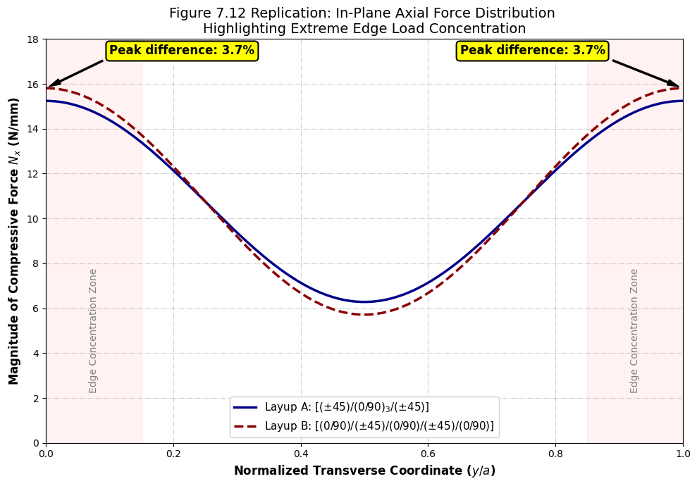
- Kassapoglou, C. (2013). Design and Analysis of Composite Structures: With Applications to Aerospace Structures. Wiley. 10.1002/9781118536933