Virtual Material Model (VMM)
Introduction
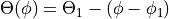
The basic problem with laminated cones is the change of the local fiber angle
due to the plane ply parts and the curved cone surface. Because of the curved
surface the fibers are lying on the geodesic path, see Figure 1. There are two
different fiber angles  and
and  at the positions
  and
and  . The variable s is part of the conical coordinate system. Goldfeld
[goldfeld2007] describes the local fiber angle
. The variable s is part of the conical coordinate system. Goldfeld
[goldfeld2007] describes the local fiber angle  as a function of s:
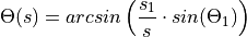
This approach is only valid for the path of a single fiber. A new approach is to describe the local fiber angle by the difference between the angle of the point of interest and the angle of the starting point of the ply part:
This approach can be used for ply parts with a finite width and is the key formula for this program.
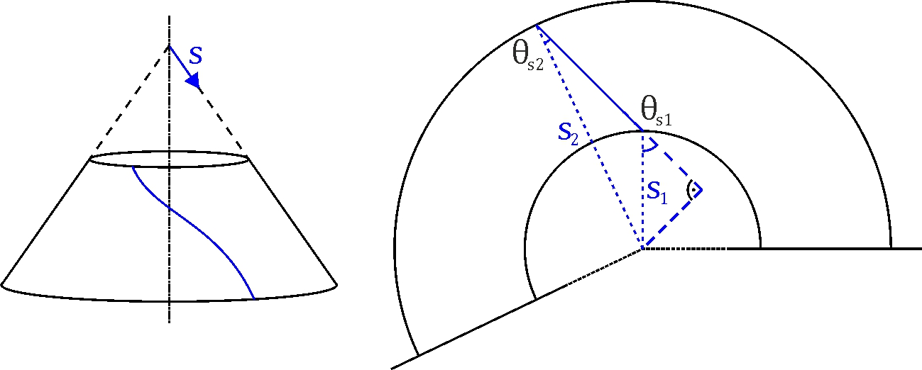
Figure 1: Path of Fiber on Cone
The objective of this tool is to calculate the local fiber angle and thickness
of any given point on a laminated cone. To do this the laminate will be
rebuilt as a virtual model. Each ply (i) consists of a finite number of pieces
(j) with a certain ply angle  and offset angle
  . These
are called ply pieces. After building the model, another algorithm determines
in which ply piece(s) a given point lies and calculates the local fiber angles
and thickness.
. These
are called ply pieces. After building the model, another algorithm determines
in which ply piece(s) a given point lies and calculates the local fiber angles
and thickness.
This manual is supposed to explain the VMM. The corresponding code is located
in desicos.cppot.core. This material model is used by both the
Abaqus-plugin (desicos.abaqus.imperfections.ppi.PPI)
and in the separate Cone Ply Piece Optimization Tool (CPPOT).
Coordinate systems
This program works with several different coordinate systems:
3D-Cartesian: Used for the model generation in ABAQUS
![x,y,z \in [-\infty, +\infty]](../../../_images/math/ff7e768ca6eb9cba71b3ab25d2854a93e19488af.png)
Figure 2: Global 3D-Cartesian coordinate system
3D-cylindrical: This often allows considerable simplification in axisymmetric cases, such as cones. Note that the symbol
 is used here
for the circumferential coordinate instead of
is used here
for the circumferential coordinate instead of  , because the latter
will be used for the fiber angle.
, because the latter
will be used for the fiber angle.
![r &\in [0, +\infty] \\
\psi &\in [0, 2\pi) \\
z &\in [-\infty, +\infty]](../../../_images/math/f9752f892f68437316abd3eb27107cb77c190cfc.png)
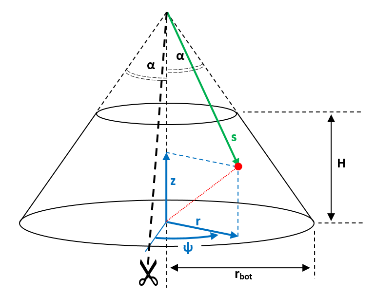
Figure 3: Global 3D-cylindrical coordinate system
The coordinate transformation between Cartesian and cylindrical coordinates and vice versa is done as follows:
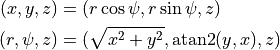
Unfolded coordinates
The cone surface is a two-dimensional surface within the three-dimensional space. Points on the cone have to satisfy the following equation:
Points that satisfy this equation can be described using a two-dimensional
coordinate system. For this purpose, an imaginary cut is made through the cone
at  , see the above figure. The apex of the cone is placed at the
origin of the new coordinate system. The edge in the direction
, see the above figure. The apex of the cone is placed at the
origin of the new coordinate system. The edge in the direction  (right edge in the figure) is mapped to the horizontal axis. This results
in the layout shown below:
(right edge in the figure) is mapped to the horizontal axis. This results
in the layout shown below:
Figure 4: Unfolded coordinate systems (polar and Cartesian)
These unfolded coordinates can be described using two coordinate systems:
2D-polar: This is the most natural description:
![s &\in [0, +\infty] \\
\phi &\in [0, \phi_{max})](../../../_images/math/35f57394c7849827e0aa9d14027b57ba74764e77.png)
The relation between the 2D-polar coordinates  and 3D-cylindrical
coordinates is as follows, valid only for points on the cone surface:
and 3D-cylindrical
coordinates is as follows, valid only for points on the cone surface:
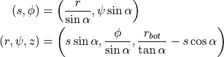
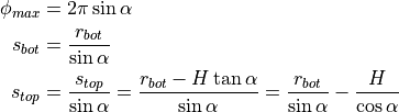
Using the above coordinate transformation, the maximum value for the
 -coordinate (labeled
  ) can be calculated, as well as the
radial limits
) can be calculated, as well as the
radial limits  and
and  :
:
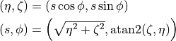
2D-Cartesian: Used for geometrical operations on the unfolded cone (defining lines, calculating intersection points, …):
![\eta, \zeta \in [-\infty,+\infty]](../../../_images/math/6bd81352562da08bcfde34261132b3d784c1e211.png)
The transformation rules are fairly straightforward:
Laminate coordinates To describe the orientation of fibers and plies, a laminate coordinate system is used in Abaqus, as is shown in the figure below. This is a local coordinate system that defines three directions at each point on the cone. The 1-direction is obtained by projecting the z-axis onto the cone surface, i.e. it is always pointing towards the apex of the cone. The n-direction is normal to the surface and always pointing outward. The 2-direction is obtained by rotating the 1-direction
 around the normal vector, using the right-hand rule. The angle
is used to define the orientation of a fiber or ply. It is defined
as being 0 for fibers parallel to the 1-direction and increases when
rotating from the 1- to 2-direction, as shown in the figure.
around the normal vector, using the right-hand rule. The angle
is used to define the orientation of a fiber or ply. It is defined
as being 0 for fibers parallel to the 1-direction and increases when
rotating from the 1- to 2-direction, as shown in the figure.
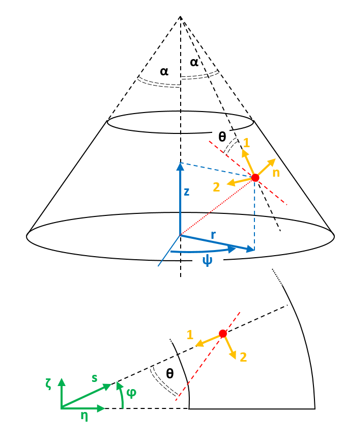
Figure 5: Laminate coordinate system, shown relative to both global (top) and unfolded (bottom) coordinates.
Detailed cone geometry
The cone geometry used in the DESICOS project is slightly more complex than the elementary truncated cone discussed in the previous chapter. Apart from the free cone area, additional support parts are present along both edges, as shown in the figure below. The support areas will be partially cut away (to obtain straight, clean edges) after laminating and the rest will be molded in resin. These areas do need to be considered when discussing the ply placement process, however.
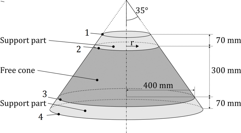
Figure 6: Example of cone geometry.
Translating this geometry to the unfolded cone results in the figure below. There are four relevant radii, labelled s1 to s4. These correspond to the edges numbered 1 to 4 in figure 6. The total area between the dotted arcs (s1 and s4) will need to be covered with ply pieces. However, only the area between the solid arcs (s2 and s3) will be relevant when determining the local fiber orientation at a later stage.
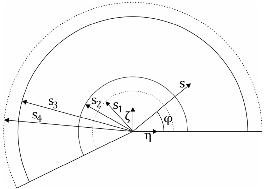
Figure 7: Radii used in unfolded cone.
In the code, the geometry of the cone is encapsulated in the
desicos.cppot.core.geom.ConeGeometry class. This class is constructed
based on a few input parameters, listed below. All other parameters
(s1 .. s4, rtop, …) are then easily retrieved upon request.
The bottom radius of the free cone
(400 mm in figure 6)
The semi-vertex angle
(
in figure 6)
The free cone height
(300 mm in figure 6)
The support height
extra_height(70 mm in figure 6)
Building the Ply model
The VMM is the virtual model of the lay-up of the laminated cone. Every ply consists of a finite number of pieces. Between the parts are no gaps, depending on the ply piece geometry there may be overlaps. In the Abaqus-plugin only one type of ply piece is available:
Type A: Trapezoidal ply pieces without overlaps
Two additional shapes are accessible through the CPPOT-program:
Type B: Trapezoidal ply pieces with one overlap
Type C: Rectangular ply pieces with many overlaps.
In this document, only shape A will be discussed, because it is the only one that has actually been used in the manufacturing of cones.
The basic process flow for building the model for a single ply is:
Construct a prototype piece
Copy and rotate the prototype piece to fill the entire cone
Calculate the local fiber orientation at the desired points
The three numbered steps will now be discussed sequentially:
1. Constructing the prototype piece
The construction of a single ply piece will now be described step-by-step.
Objective is mainly to describe the procedure, not to bother the reader with
implementation details (e.g. “How to find the intersection of two lines?”). For
the latter, consult the relevant pieces of code. The implementation of the
procedure described here is contained in the method
desicos.cppot.core.ply_model.TrapezPlyPieceModel.construct_single_ply_piece().
The constructed ply pieces will be trapezoidal in shape, as shown in the
figure below. These trapezoidal pieces will be constructed such the angle that
is spanned or “covered” by each ply piece is a constant  ,
independent of
,
independent of  . This property is important to allow covering the entire
cone with similarly-shaped pieces, without having gaps or overlaps.
. This property is important to allow covering the entire
cone with similarly-shaped pieces, without having gaps or overlaps.
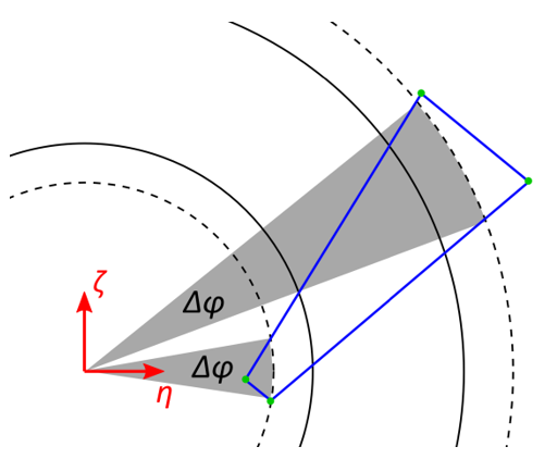
Figure 8: View of single ply piece
Step 1: Origin line `L_0`
The first step is to construct the origin line  . All fibers in the ply
piece will be parallel to this line. It is defined based on three parameters:
. All fibers in the ply
piece will be parallel to this line. It is defined based on three parameters:
The nominal fiber angle
 , which is the same for all ply pieces
in a ply.
, which is the same for all ply pieces
in a ply.The nominal ply piece angle
 . Note that this is a property of the
individual ply piece, not a property of the ply.
. Note that this is a property of the
individual ply piece, not a property of the ply.The starting position
 , which is the radius at which
(at the nominal ply piece angle ) the actual fiber angle equals
the nominal fiber angle.
, which is the radius at which
(at the nominal ply piece angle ) the actual fiber angle equals
the nominal fiber angle.
The line is then defined as the line going through the point
 at an angle
(
at an angle
( ) with respect to the
  -axis. See figure 9:
Figure 9: Construction of origin line 
Step 2: Base line `L_2`
The base line  is the line along which the width of the ply piece will
be measured. is defined as the line perpendicular to and tangent to
the circle with radius
is the line along which the width of the ply piece will
be measured. is defined as the line perpendicular to and tangent to
the circle with radius  . Point
  is then defined as the intersection
point of and . See Figure 10:
is then defined as the intersection
point of and . See Figure 10:
Figure 10: Construction of base line 
Step 3: Corners at outer edge
The outer edge of the polygon is formed by the line . The position of the
corner points  and
and  along this line is determined by two parameters:
The maximum ply piece width
 is equal to the distance between the
two points and .
is equal to the distance between the
two points and .The eccentricity parameter
 (also known as width variation)
determines the placement of the two points relative to . is
defined as the distance from to , divided by . So for
(also known as width variation)
determines the placement of the two points relative to . is
defined as the distance from to , divided by . So for
 , and coincide and for
  , and
coincide.
, and
coincide.
This is also shown in figure 11. So is defined as the point on at a
distance ( ) from , while is defined as the
point on at a distance (
) from , while is defined as the
point on at a distance ( ) from .
For completeness, it should be mentioned that is to be placed in the
counter-clockwise direction relative to and in the clockwise
direction relative to , as is evident in the figure below.
) from .
For completeness, it should be mentioned that is to be placed in the
counter-clockwise direction relative to and in the clockwise
direction relative to , as is evident in the figure below.
Figure 11: Construction of and 
Step 4: Calculating the spanned angle
Now it is necessary to calculate the angle that is spanned by the
ply piece. This angle is determined by the position of points and .
However, it would be wrong to take the angular coordinates of and
and subtract them (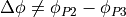 ), because the radii
 and
and  of these points are not the same.
Therefore, the points  and
and  are constructed first. Point
  is
defined as the point lying on at a distance
is
defined as the point lying on at a distance  from the origin.
Now the two constituent parts of can be calculated. One part is
the difference in angular coordinate between and , the other between
and . This is shown more clearly in figure 12 below.
from the origin.
Now the two constituent parts of can be calculated. One part is
the difference in angular coordinate between and , the other between
and . This is shown more clearly in figure 12 below.
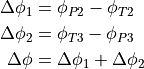
Figure 12: Angle spanned by ply piece
Step 5: Constructing the side lines
Now the side lines  and
and  can be constructed by rotating around
the origin. is constructed by rotating counter-clockwise with angle
can be constructed by rotating around
the origin. is constructed by rotating counter-clockwise with angle
 , is constructed by rotating clockwise around angle
 .The intersection point between and circle is
denoted as
.The intersection point between and circle is
denoted as  , the intersection point between and circle is
denoted as
, the intersection point between and circle is
denoted as  . All of this is shown in figure 13:
Figure 13: Constructing the side lines and 
Step 6: Corners at the inner edge
Now the inner edge of the polygon is to be defined. First, it is examined which
point is further from , either or . See figure 14, in
the shown example case the point is the furthest from . The line
 is then defined to be parallel to and through this furthest point.
Then points
is then defined to be parallel to and through this furthest point.
Then points  and
and  are defined as the intersection points of with,
respectively, and .
are defined as the intersection points of with,
respectively, and .
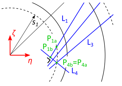
Figure 14: Constructing 
There is a special case, which is shown in figure 15. Namely, for some
combinations of parameters, the previous procedure may lead to polygons
(,  ,
,  , ) that are self-intersecting. In this
case, both
, ) that are self-intersecting. In this
case, both  and
and  are defined to be equal to the intersection point of
and and the ply piece becomes a triangle. This results in some very
small areas along circle being not covered with any ply piece. This is
deemed acceptable, because the area between and is not relevant for
the finite element model.
are defined to be equal to the intersection point of
and and the ply piece becomes a triangle. This results in some very
small areas along circle being not covered with any ply piece. This is
deemed acceptable, because the area between and is not relevant for
the finite element model.
In the normal case of figure 14, where the polygon is not self-intersecting,
the final locations of and are equal to and ,
respectively.
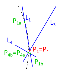
Figure 15: Special case for triangular ply piece
Step 7: Final ply piece
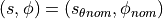
The final shape of the ply piece is shown in figure 16 below. Its shape is
defined by the four corner points  . On the circle with radius
(the starting position), the ply piece spans an angle from
. On the circle with radius
(the starting position), the ply piece spans an angle from
 to
to  . These angles can be calculated by:
Additionally, the limit angles of the ply piece are defined as the minimal and maximum value of the angular coordinate. Since the extreme values are always located at the corner points, these can be calculated by:
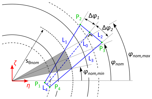
Figure 16: Final ply piece
2. Constructing all ply pieces
Based on the prototype ply piece discussed in the previous section, the
complete set of ply pieces can be constructed. In the code, this is implemented
mainly in the method
desicos.cppot.core.ply_model.PlyPieceModel.rebuild().
First the required number of ply pieces is determined:
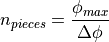
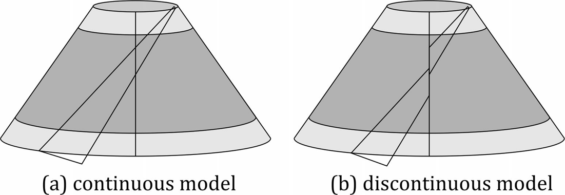
Figure 17: Continuity problem
Generally,  is not an integer, so covering the entire cone with
similar pieces would result in a discontinuous model, as shown in figure 17.
To remedy this problem, a smaller rest piece is added. This rest piece should
span an angle: (with
is not an integer, so covering the entire cone with
similar pieces would result in a discontinuous model, as shown in figure 17.
To remedy this problem, a smaller rest piece is added. This rest piece should
span an angle: (with  denoting the floor function)
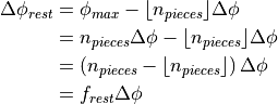
with
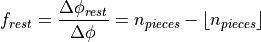
So in words,  is the fractional part of . To construct
the rest piece, the same procedure is followed as for a normal ply piece.
However, during step 4, the calculated values of and
are multiplied by as stated below. This results in
a ply piece whose angular span
is the fractional part of . To construct
the rest piece, the same procedure is followed as for a normal ply piece.
However, during step 4, the calculated values of and
are multiplied by as stated below. This results in
a ply piece whose angular span  satisfies the above
equations. The positions of points and (and, of course, the
calculations in subsequent steps) are adjusted accordingly.
satisfies the above
equations. The positions of points and (and, of course, the
calculations in subsequent steps) are adjusted accordingly.
Now the procedure to cover the entire cone with ply pieces is as follows. The
first piece is placed at a nominal angle equal to  .
This is done to allow offsettnig multiple plies with the same nominal fiber
orientation with respect to each other. This avoids that the ply piece
edges in multiple plies coincide, which would (unnecessarily) cause weak spots
in the actual cone. The offset parameter is specified in relative terms
(0…1), based on this value is calculated as follows:
.
This is done to allow offsettnig multiple plies with the same nominal fiber
orientation with respect to each other. This avoids that the ply piece
edges in multiple plies coincide, which would (unnecessarily) cause weak spots
in the actual cone. The offset parameter is specified in relative terms
(0…1), based on this value is calculated as follows:
Ply pieces are then placed in both directions at angular increments of
 . Pieces are added as long as they cover some area in the
angular range
. Pieces are added as long as they cover some area in the
angular range ![[0, \phi_{max}]](../../../_images/math/6eb3130593c2579a91cd6af8217f8eff861b6de9.png) , which is the case if both below-stated
inequalities are satisfied.
, which is the case if both below-stated
inequalities are satisfied.
The possible result of this operation is shown in figure 18. Here the unfolded
cone is drawn in red, the first ply piece in blue, the other ply pieces in
green and the nominal angle of each ply piece as a dashed black line. The rest
piece is inserted right after (in counter-clockwise direction) the first piece
for which  . This prevents the rest piece from overlapping
the “cut” in the model, which would add additional complexity to the model.
Some special handling is needed to set the angular offsets between the rest
piece and its neighboring pieces. If the nominal angles of the rest piece,
the previous piece and the next piece are named
. This prevents the rest piece from overlapping
the “cut” in the model, which would add additional complexity to the model.
Some special handling is needed to set the angular offsets between the rest
piece and its neighboring pieces. If the nominal angles of the rest piece,
the previous piece and the next piece are named  ,
,
 and
and  , respectively, their mutual relations
are as stated below. Refer also to the figure.
, respectively, their mutual relations
are as stated below. Refer also to the figure.
Figure 18: Covering the cone
Note that the model contains a few more ply pieces than the actual cone,
because the pieces that intersect the cut ( and
and  )
are represented twice. This is done because it simplifies the implementation,
while not affecting the results in any way.
)
are represented twice. This is done because it simplifies the implementation,
while not affecting the results in any way.
3. Calculating the local orientation
To calculate what the local fiber angle is at any point on the cone, several steps are needed.
Step 1: Change coordinate system
First, the coordinates in the global coordinate system have to be transformed
to the coordinates of the unfolded cone, i.e.  and/or
. These coordinate transformations have been discussed in a
previous chapter on this page and will not be repeated.
and/or
. These coordinate transformations have been discussed in a
previous chapter on this page and will not be repeated.
Step 2: Find the correct ply piece
Next, it is necessary to find the ply piece(s) located at the given coordinates. This is done by iterating over all ply pieces and then,for each ply piece:
Quickly check whether
 .
If not, continue.
.
If not, continue.Perform the (computationally more expensive) test whether the point is inside the polygon that defines this ply piece. In earlier versions the “interior angle”-algorithm was used, but for performance reasons this was changed to the “ray casting”-algorithm. Both algorithms are widely used and extensively documented in other sources. If this check returns a positive result, stop iteration and return this ply piece. If not, continue.
If iteration completes without having found a ply piece, the point is not on the cone at all and
NaNis returned.
Step 3: Find the local angle
A relation for the local fiber angle can be found, based on the principle that
the sum of all angles inside a triangle is always equal to  . This
results in the following equation:
. This
results in the following equation:

An example plot of the local fiber angle is shown in the figure below. Note
that all points within the same ply piece have a constant fiber angle along
radial lines ( ) and that there are significant
discontinuities between adjacent plies.
) and that there are significant
discontinuities between adjacent plies.
Figure 18: Example of local fiber orientation throughout the cone