Processing Geometric Imperfection Data

This part of the turorial will explain in a step-by-step example how one can use the developed modules to post-process measured imperfection data.

The following steps will be discussed:

• raw data from measurement system

• finding

Raw Data from Mesurement Systems

The raw files obtained from measured geometric imperfections usually come with three columns:

x1 y1 z1
x2 y2 z2
...
xn yn zn

The following sample has been used to illustrate this tutorial (first 10 lines shown below):

310.909   1174.136   261.8
146.126   754.321   378.119
216.694   1111.78   342.928
-261.395   1031.417   -314.052
-5.499   99.519   -407.764
-70.556   95.452   -401.672
-336.88   1148.365   -229.665
-351.651   705.414   204.226
403.703   454.238   -37.619
122.444   55.322   386.451

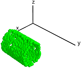
The following script is used to plot the sample with the imperfection exagerated. Note that best_fit_raw_data.py has to be executed before.

plot_sample_3d.py

import numpy as np
import mayavi.mlab as mlab

from desicos.conecylDB.read_write import xyz2thetazimp

R = 406.4 # nominal radius
H = 1219.2 # nominal height
R_best_fit = 407.193 # radius obtained with the best-fit routine

thetas, zfit, dR = np.genfromtxt('sample_theta_z_imp.txt', unpack=True)

xpos = R_best_fit*np.cos(thetas)
ypos = R_best_fit*np.sin(thetas)
sf = 20
x2 = xpos + sf*dR*np.cos(thetas)
y2 = ypos + sf*dR*np.sin(thetas)
z2 = zfit

Tinv = np.loadtxt('tmp_Tinv.txt')
x, y, z = Tinv.dot(np.vstack((x2, y2, z2, np.ones_like(x2))))

black = (0,0,0)
white = (1,1,1)
mlab.figure(bgcolor=white)
mlab.points3d(x, y, z, color=(0,1,0))
mlab.plot3d([0, 600], [0, 0], [0, 0], color=black, tube_radius=10.)
mlab.plot3d([0, 0], [0, 1600], [0, 0], color=black, tube_radius=10.)
mlab.plot3d([0, 0], [0, 0], [0, 600], color=black, tube_radius=10.)
mlab.text3d(650, -50, +50, 'x', color=black, scale=100.)
mlab.text3d(0, 1650, +50, 'y', color=black, scale=100.)
mlab.text3d(0, -50, 650, 'z', color=black, scale=100.)
mlab.savefig('plot_sample_3d.png', size=(500, 500))

giving:

In order to transform the raw data to the finite element coordinate system, the recommended procedure is the function xyz2thetazimp(), exemplified below. This function converts the “ ” data to a to convert them to a “ ” format. This function is a wrapper that calls funcion best_fit_cylinder() or best_fit_cone(), where the right coordinate transformation is calculated.

best_fit_raw_data.py

import numpy as np

from desicos.conecylDB.read_write import xyz2thetazimp

mps, out = xyz2thetazimp('sample.txt', alphadeg_measured=0, R_expected=406.4,
        H_measured=1219.2, clip_bottom=10, clip_top=10, use_best_fit=True,
        best_fit_output=True, rotatedeg=0.)

np.savetxt('tmp_Tinv.txt', out['Tinv'])

It will create an output file with a prefix "_theta_z_imp.txt" where the imperfection data is stored in the format:

theta1 z1 imp1
theta2 z2 imp2
...
thetan zn impn

where thetai and zi are the coordinates and , while impi represents the imperfection amplitude at this coordinate. An example of the transformed imperfection data is given below (first 10 lines), and the full output is given here:

0.701704 44.752223 -0.299107
1.202029 464.737892 -0.772438
1.008550 107.201740 -0.834017
-2.266294 188.347008 0.697946
-1.581399 1119.953672 -0.574269
-1.742285 1124.099646 -0.728166
-2.545140 71.468489 0.131696
2.612788 514.312597 -0.417002
-0.090133 764.620654 -1.094824
1.261926 1163.763315 -0.307154

Note

It is also possible to use xyz2thetazimp() in other ways, as detailed in the function’s documentation

The transformed data can also be visualized in the 3-D domain, which was accomplished using the following script:

plot_sample_3d_tranformed.py

import numpy as np
import mayavi.mlab as mlab

from desicos.conecylDB.read_write import xyz2thetazimp

R = 406.4
R_best_fit = 407.168

data = np.genfromtxt('sample_theta_z_imp.txt')
thetas, zfit, dR = data.T

xpos = R_best_fit*np.cos(thetas)
ypos = R_best_fit*np.sin(thetas)
sf = 20
x2 = xpos + sf*dR*np.cos(thetas)
y2 = ypos + sf*dR*np.sin(thetas)
z2 = zfit

black = (0,0,0)
white = (1,1,1)
mlab.figure(bgcolor=white)
mlab.points3d(x2, y2, z2, color=(0.5,0.5,0.5))
mlab.plot3d([0, 600], [0, 0], [0, 0], color=black, tube_radius=10.)
mlab.plot3d([0, 0], [0, 600], [0, 0], color=black, tube_radius=10.)
mlab.plot3d([0, 0], [0, 0], [0, 1600], color=black, tube_radius=10.)
mlab.text3d(650, -50, +50, 'x', color=black, scale=100.)
mlab.text3d(0, 650, +50, 'y', color=black, scale=100.)
mlab.text3d(0, -50, 1650, 'z', color=black, scale=100.)
mlab.savefig('plot_sample_3d_transformed.png')

giving:

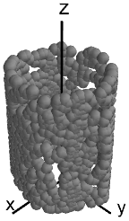
Note that due to the axisymmetry it may happen that the final result has some offset rotation. For this reason the interpolation routines that will be discussed in the next sessions of this tutorial include a rotatedeg parameter that the analyst should use in order to correct this angular offset.

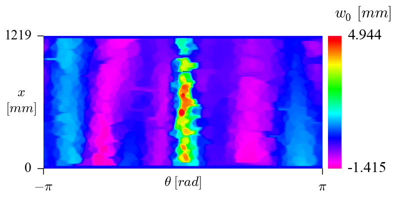
Inverse-Weighted Interpolation

Function iterp_theta_z_imp() is the one used to interpolate the measured data into a given mesh. In the example below the mesh creates using np.meshgrid() is used for plotting purposes. Note that the an angular offset of -88.5 degrees was used in order to adjust the imperfection.

interpolate_inv_weighted.py

import numpy as np

from desicos.conecylDB.interpolate import interp_theta_z_imp

R_model = 406.4 + 0.8128/2.
H_measured = 1219.2
ignore_bot_h = 25.4
ignore_top_h = 25.4

nz = 180
nt = 560

theta = np.linspace(-np.pi, np.pi, nt)
z = np.linspace(0, H_measured, nz)
T, Z = np.meshgrid(theta, z, copy=False)

data = np.loadtxt('sample_theta_z_imp.txt')
ts, zs, imps = data.T
a = np.vstack((ts, zs, imps)).T
mesh = np.vstack((T.ravel(), Z.ravel())).T
w0 = interp_theta_z_imp(data=a, mesh=mesh, semi_angle=0,
        H_measured=H_measured, H_model=H_measured, R_model=R_model,
        stretch_H=False, rotatedeg=-88.5, num_sub=100, ncp=5,
        power_parameter=2, ignore_bot_h=ignore_bot_h,
        ignore_top_h=ignore_top_h)
np.savetxt('tmp_inv_weighted.txt',
           np.vstack((T.ravel(), Z.ravel(), w0)).T, fmt='%1.8f')

An the generated data can be plotted using the following code:

plot_inv_weighted.py

import numpy as np
from numpy import pi
import matplotlib.cm as cm
import matplotlib.pyplot as plt

plt.rcParams['axes.labelsize'] = 9.
plt.rcParams['font.size'] = 9.

path = 'tmp_inv_weighted.txt'

nz = 180
nt = 560

R = 407.168

#cmap = cm.jet
cmap = cm.gist_rainbow_r

theta, z, w0 = np.loadtxt(path, unpack=True)

fig = plt.figure(figsize=(3.5, 3.5), dpi=220)
levels = np.linspace(w0.min(), w0.max(), 400)
contour = plt.contourf(theta.reshape(nz, nt)*R, z.reshape(nz, nt),
        w0.reshape(nz, nt), levels=levels, cmap=cmap)

ax = plt.gca()
ax.xaxis.set_ticks_position('bottom')
ax.yaxis.set_ticks_position('left')
ax.spines['top'].set_visible(False)
ax.spines['right'].set_visible(False)
ax.spines['bottom'].set_visible(False)
ax.spines['left'].set_visible(False)

ax.set_aspect('equal')
ax.xaxis.set_ticks([-pi*R, pi*R])
ax.xaxis.set_ticklabels([r'$-\pi$', r'$\pi$'])
ax.set_xlabel(r'$\theta$ $[rad]$', ha='center', va='center')
ax.xaxis.labelpad=-7

ax.yaxis.set_ticks([0, 1219.2])
ax.set_ylabel('$x$\n$[mm]$', rotation='horizontal', ha='center',
        va='center')
ax.yaxis.labelpad=-10

colorbar=True
if colorbar:
    from mpl_toolkits.axes_grid1 import make_axes_locatable

    fsize = 10
    cbar_nticks = 2
    divider = make_axes_locatable(ax)
    cax = divider.append_axes('right', size='5%', pad=0.05)
    cbarticks = np.linspace(w0.min(), w0.max(), cbar_nticks)
    cbar = plt.colorbar(contour, ticks=cbarticks, format='%1.3f',
                        cax=cax, cmap=cmap)
    cax.text(0.5, 1.1, '$w_0$ $[mm]$', ha='left', va='bottom',
            fontsize=fsize)
    cbar.outline.remove()
    cbar.ax.tick_params(labelsize=fsize, pad=0., tick2On=False)

fig.savefig('plot_inv_weighted.png', transparent=True,
                  bbox_inches='tight', pad_inches=0.05, dpi=220)

giving:

Half-Cosine Function

Function calc_c0() is used to interpolate the measured data using Fourier series. The half-cosine function corresponds to the parameter funcnum = 2, as can be seen in the function’s documentation.

The following script was used to calculate the coefficients . Note how the angular offset is applied using the rotatedeg parameter:

interpolate_half_cosine.py

import numpy as np

from desicos.conecylDB.fit_data import calc_c0

method = 'points'
funcnum= 2

path = 'sample_theta_z_imp.txt'

R = 406.4 + 0.8128/2.
H = 1219.2
m0 = 10
n0 = 10

c0, residues = calc_c0(path, m0=m0, n0=n0, funcnum=funcnum, rotatedeg=-88.5)
outname = 'tmp_c0_{0}_f{1:d}_m0_{2:03d}_n0_{3:03d}.txt'.format(method,
        funcnum, m0, n0)
np.savetxt(outname, c0)

and the following routine was used to plot the corresponding imperfection field:

plot_half_cosine.py

import numpy as np
from numpy import pi
import matplotlib.cm as cm
import matplotlib.pyplot as plt

from compmech.conecyl.imperfections import fw0

plt.rcParams['axes.labelsize'] = 9.
plt.rcParams['font.size'] = 9.

method = 'points'
funcnum = 2
names = ['C01']

nz = 180
nt = 560

H = 1219.2
zpts_min = 25.4
zpts_max = H - 25.4
R = 406.4 + 0.8128/2.

#cmap = cm.jet
cmap = cm.gist_rainbow_r

m0 = 10
n0 = 10

filename = 'tmp_c0_{0}_f{1:d}_m0_{2:03d}_n0_{3:03d}.txt'.format(method,
        funcnum, m0, n0)
c0 = np.loadtxt(filename)
ts = np.linspace(-pi, pi, nt)
xs = np.linspace(0, 1., nz)
zs = xs*H
check = (zs >= zpts_min) & (zs <= zpts_max)
test = xs[check]
xs -= test.min()
xs /= xs.max()
xs[xs<0] = 0
xs[xs>1] = 1

dummy, xs = np.meshgrid(ts, xs, copy=False)
ts, zs = np.meshgrid(ts, zs, copy=False)

w0 = fw0(m0, n0, c0, xs, ts, funcnum=funcnum)
w0.flat[(zs.flat < zpts_min) | (zs.flat > zpts_max)] = 0

fig = plt.figure(figsize=(3.5, 3.5), dpi=220)

levels = np.linspace(w0.min(), w0.max(), 400)
contour = plt.contourf(ts*R, zs, w0.reshape(ts.shape), levels=levels,
        cmap=cmap)

ax = plt.gca()
ax.set_aspect('equal')
ax.xaxis.set_ticks_position('bottom')
ax.yaxis.set_ticks_position('left')
ax.spines['bottom'].set_visible(False)
ax.spines['top'].set_visible(False)
ax.spines['left'].set_visible(False)
ax.spines['right'].set_visible(False)

ax.xaxis.set_ticks([-pi*R, pi*R])
ax.xaxis.set_ticklabels([r'$-\pi$', r'$\pi$'])
ax.set_xlabel(r'$\theta$ $[rad]$', va='center', ha='center')
ax.xaxis.labelpad = -7

ax.yaxis.set_ticks([0, H])
ax.set_ylabel('$z$\n$[mm]$', rotation='horizontal', va='center',
        ha='center')
ax.yaxis.labelpad = -10


colorbar = True
if colorbar:
    from mpl_toolkits.axes_grid1 import make_axes_locatable

    fsize = 10
    cbar_nticks = 2
    divider = make_axes_locatable(ax)
    cax = divider.append_axes('right', size='5%', pad=0.05)
    cbarticks = np.linspace(w0.min(), w0.max(), cbar_nticks)
    cbar = plt.colorbar(contour, ticks=cbarticks, format='%1.3f',
                        cax=cax, cmap=cmap)
    cax.text(0.5, 1.1, '$w_0$ $[mm]$', ha='left', va='bottom',
            fontsize=fsize)
    cbar.outline.remove()
    cbar.ax.tick_params(labelsize=fsize, pad=0., tick2On=False)

fig.savefig('plot_half_cosine.png', transparent=True, bbox_inches='tight',
        pad_inches=0.05, dpi=220)

giving:

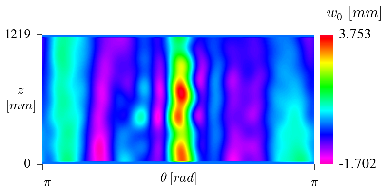
The relatively poor correlation between the half-cosine and the inverse_weighted is primarily due to the reduced amount of measured data used for this tutorial. Using real imperfection data the correlation is much closer, as shown in the additional examples below.

Additional Examples using the Half-Cosine Function

The example below shows how to use this function and then plot the displacement patterns using different approximation levels:

half_cosine_additional_example.py

from numpy import *

from desicos.conecylDB.fit_data import fw0

ntheta = 420
nz = 180
funcnum = 2
path = 'degenhardt_2010_z25_msi_theta_z_imp.txt'

theta = linspace(-pi, pi, ntheta)
z = linspace(0., 1., nz)
theta, z = meshgrid(theta, z, copy=False)

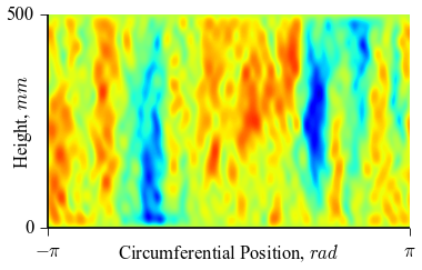
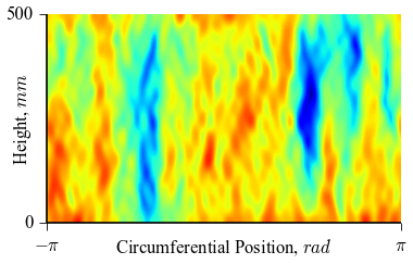
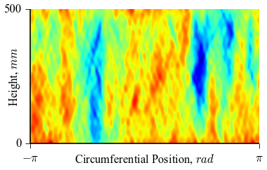
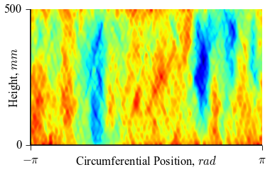
for m0, n0 in [[20, 30], [30, 45], [40, 60], [50, 75]]:
    c, residues = calc_c0(path, m0=m0, n0=n0, sample_size=(10*2*m*n),
                          funcnum=funcnum)

    w0 = fw0(m0, n0, z.ravel(), theta.ravel(), funcnum=funcnum)

    plt.figure(figsize=(3.5, 2))

    levels = np.linspace(w0.min(), w0.max(), 400)
    plt.contourf(theta, z*H_measured, w0.reshape(theta.shape),
                 levels=levels)

    ax = plt.gca()
    ax.xaxis.set_ticks_position('bottom')
    ax.yaxis.set_ticks_position('left')
    ax.spines['top'].set_visible(False)
    ax.spines['right'].set_visible(False)

    ax.xaxis.set_ticks([-pi, pi])
    ax.xaxis.set_ticklabels([r'$-\pi$', r'$\pi$'])
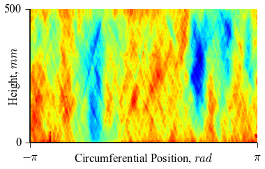
    ax.set_xlabel('Circumferential Position, $rad$')
    ax.xaxis.labelpad=-10

    ax.yaxis.set_ticks([0, 500])
    ax.set_ylabel('Height, $mm$')
    ax.yaxis.labelpad=-15

    filename = 'fw0_f{0}_z25_m_{1:03d}_n_{2:03d}.png'.format(
                funcnum, m0, n0)

    plt.gcf().savefig(filename, transparent=True, bbox_inches='tight',
                      pad_inches=0.05, dpi=90)

which will result in the following figures for funcnum=1:

, :

, :

, :

, :

and for funcnum=2:

, :

, :

, :

, :

It can be seen how the function approximates the measured imperfection pattern with the increase of and . The measured imperfection pattern is shown below, and it was plotted after performing the inverse-weighted interpolation already described.

Comparing the results using funcnum=1 and funcnum=2, one see that the latter approaches closer the real measurements, since it relaxes the condition at the edges.

Processing Measured Thickness Imperfection Data

The procedure described for geometric imperfections is also applicable for thickness imperfections. The measured imperfection data usually comes in a 4 columns format where the thickness measurement is given for each spatial position: , , :

x1 y1 z1 thick1
x2 y2 z2 thick2
...
xn yn zn thickn

The recommended procedure to transform the raw data to the finite element coordinate system is the function xyzthick2thetazthick(), that also calls internally the best_fit_cylinder() or the best_fit_cone() routines:

>>> from desicos.conecylDB.read_write import xyzthick2thetazthick

>>> xyzthick2thetazthick(path, alphadeg_measured, R_measured, H_measured,
                         fmt='%1.8f')

Note

It is possible to use function xyzthick2thetazthick`() in other ways, as detailed in the corresponding documentation