GUI

The user-friendly way to use the plug-in is through the graphic interface. Just execute the file START_GUI.bat. You need Abaqus to be executable by the command line abaqus cae for this to work.

The plug-in for Abaqus looks like this:

Loading and configuring a model

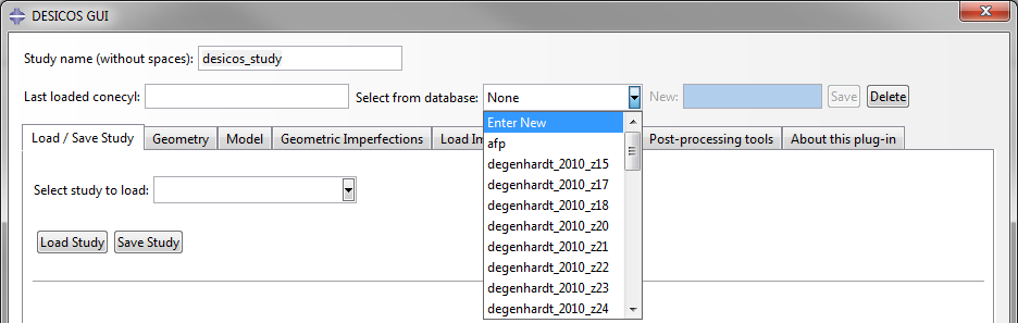
Where the desicos.conecylDB is embedded, and the existing models easily chosen from the Static Database or from the Dynamic database. When the option Enter New is active, the buttons Save is activated and the user may save a new configuration into the database, which can be deleted afterwards using the Delete button.

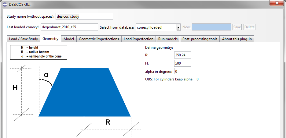
Geometric parameters easily changed:

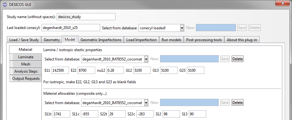
Material properties taken from the database and easily changed. Note that the Dynamic database is implemented here through the use of the buttons Save (when the Enter New option is active) and Delete.

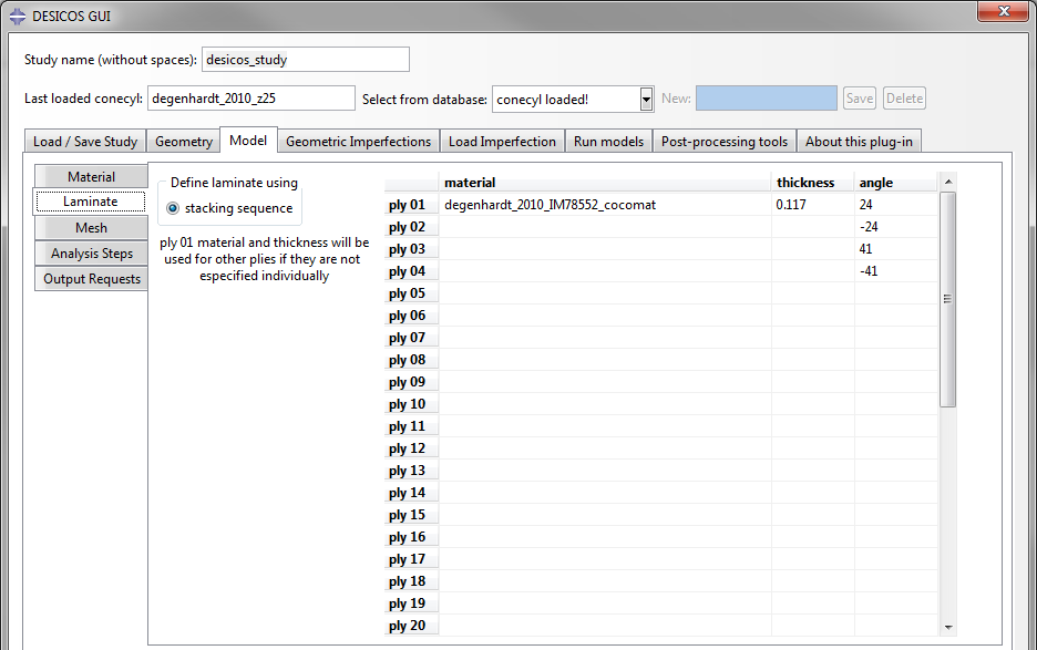
The laminate is defined giving a different material and thickness to each ply or defining only for the first ply when all the others should have the same material and thicknesses.

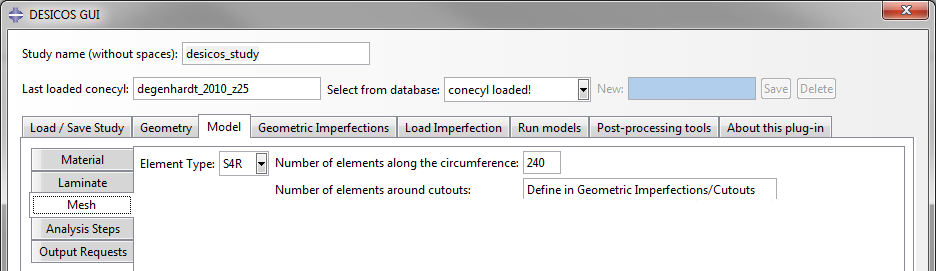
The mesh parameters are defined as shown below, and this data can also be saved and loaded in the database.

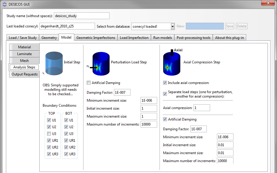
The analysis parameters are summarized as shown below. After the models are created the user may change those. This analysis’ configuration has been optimized for the Single Perturbation Load Approach (SPLA).

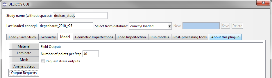
The number of output frames can be changed here, allowing some control in the size of the output files. The Request stress output checkbox must be activated if one intents to perform a stress analysis:

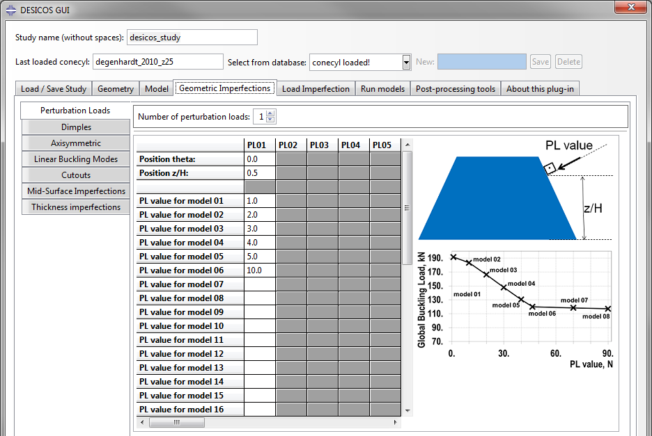
Applying imperfections

The perturbation loads can be applied using:

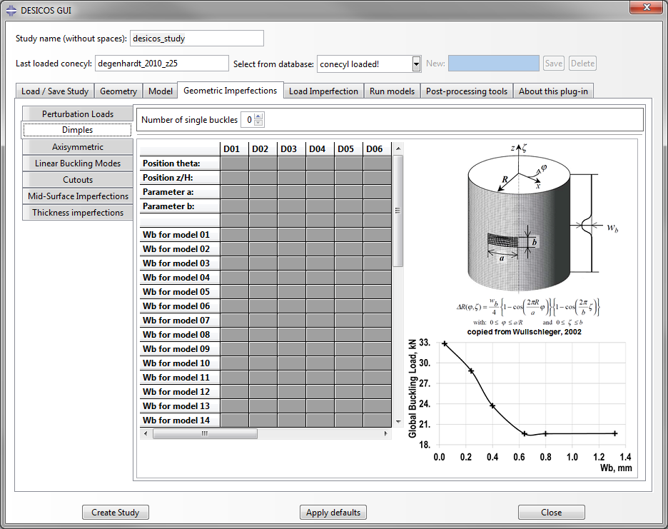
The geometric dimples using:

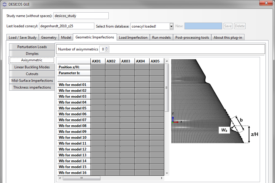
Axisymmetric imperfections:

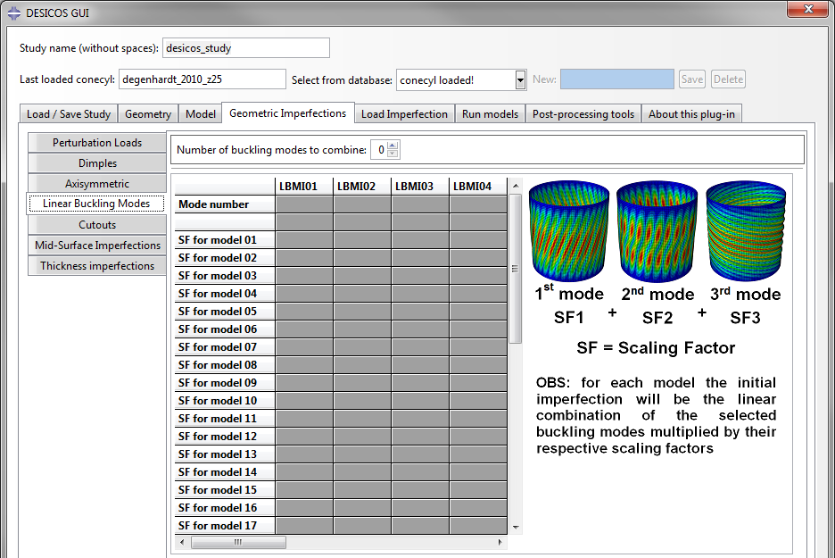
Imperfections from Linear buckling modes:

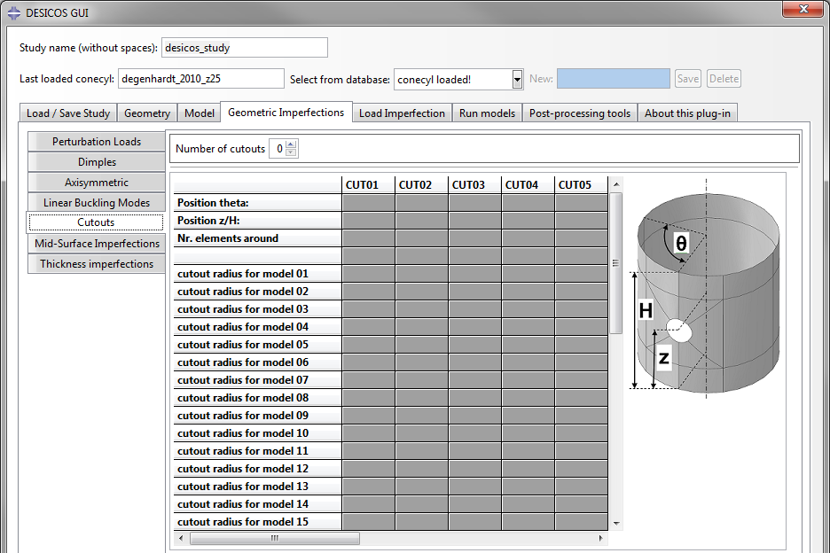
Cutouts:

Note

The cutouts module needs improvement!

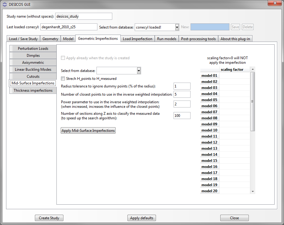
Measured geometric imperfections that represent the normal displacement of the shell mid-surface can be applied too. This must be applied after creating the study (click on Create Study):

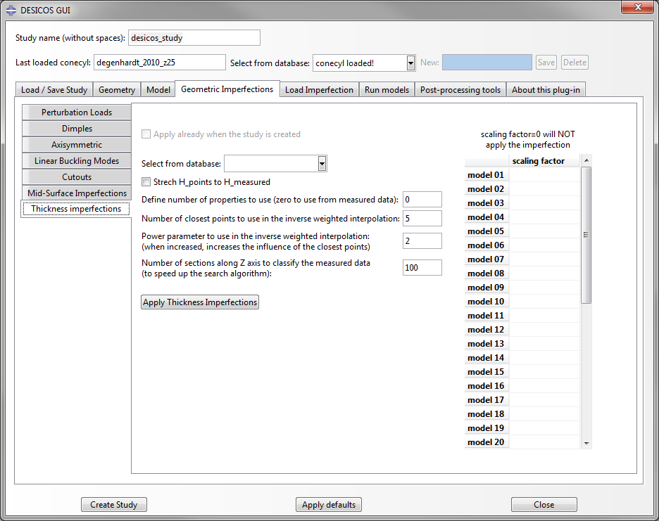
Similarly, thickness imperfections can be applied. If the study has not yet been created, click on Create Study before applying the thickness imperfections:

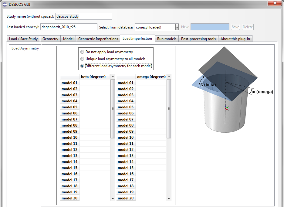
Load imperfections can also be considered:

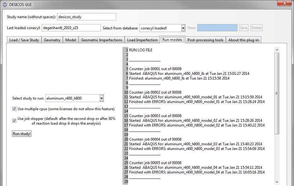
Running the analysis

It allows running the jobs in the structure of folders used by the plug-in in order to keep the models organized. You can use multiple cpus or use the job stopper, which significantly accelerates the analysis time by stopping the analysis after buckling.

If the post-buckled pattern have to be studied, it may be better to run one analysis with the job stopper activated, obtain the axial compression level that caused the buckling and then run another analysis disabling the job stopper in order to achieve the desired post-buckled pattern.

The run log file will be printed on the plug-in screen.

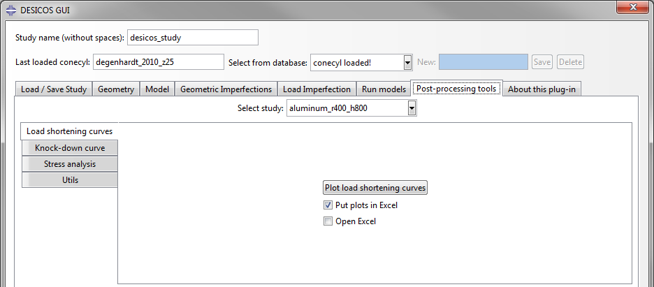
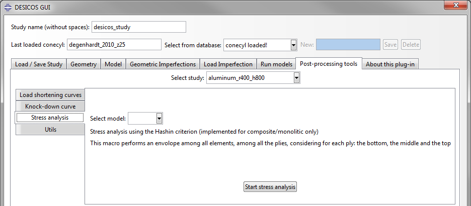
Post processing

For all the options you can add the results to an Excel file or even open the Excel after finished.

The load-shortening curves can be easily plotted:

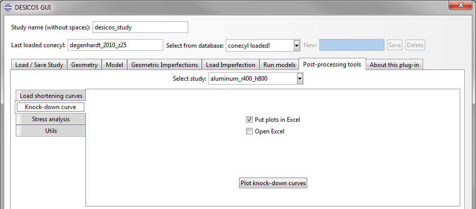
Or the knock-down curves:

Or the stress analysis results:

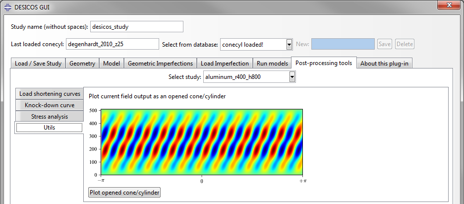
An extra options has been added to allow an opened representation of the cylinder or cone, convinient for publications: