Structural Optimization of a wingbox#
In the previous notebook we have seen the structural analysis of a single wingbox cell. We would like however to use these tools to optimize the various parameters of the wingbox in order to minimize the weight of the structure. In order to do so let’s remind ourselves what exactly we can change in order to improve the performance of this wingbox.
In the previous notebook we had defined the following parameters in order to perform the analysis.
\(n_{cell}\) - Number of cells
\(\text{loc}_{sp}\) - The location of the spars
\(t_{sk}\) - The thickness of the skin in each cell
\(A_{str}\) - The area of the stringers
\(t_{sp}\) - The thickness of the spars
\(n_{str}\) - The amount of stringers per cell
These variables were then loaded in the API data structure as shown below:
attr_dict = {
    "n_cell":4,
    "spar_loc_nondim":[0.3, 0.5, 0.7],
    "t_sk_cell":[0.002,0.004,0.004, 0.004],
    "area_str":20e-6,
    "t_sp":0.008,
    "str_cell":[8,8,7,8]
}

wingbox_struct = tud.Wingbox(**attr_dict)
However, there will be one major change. For the structural analysis of a wingbox only the stringer area is relevant however for the constraints the geometry of said stringers is also important as you will see further up in this notebook.
So in the optimization of the wingbox we wil add the stringer height, width and thickness to the optimization parameters.
The parameters which we will optimize for are the skin thickness in each cell, the area of the stringers, the thickness of the spars and finally the stringer of the cell. This leaves the amount of cells, the spar locations and the bay length to be decided by the designers. The reasoning behind this is that usually your rib and spar locations are constrained the placement of other systems in the wing such as the flap and slat mechanism. Below a summary can be found of the fixed and optimization parameters:
Optimiziation Parameters |
Fixed Parameters |
|---|---|
Skin thickness in each cell |
The amount of cells |
Stringer width |
Spar locations |
Stringer height |
Bay length |
Stringer thickness |
|
Spar thickness |
|
The amount of stringers in each cell |
Laying out a framework for a full wing optimization#
In order define our constraints later on we will have to divide the wing in sections called bays. Each bay is enclosed by two ribs, thus the length of these bays is for the designer to decide. Once, a bay is defined, we can further split this up in a collection of flat sheets. Where each sheet is in turn enclosed by stringers. The boundary conditions for these stringers have been decided to be simply supported. In figure 1 we can see the result of the partitioning that was just described. Although we will not model the effects of taper (Future implementation).

Figure 1: Wing modeled as a combination of simply supported sheets and simply supported bays. Figure taken from T.H.G Megson, Aircraft Structures For Engineering Students
Now that our wing has been divided into bays, and the bays respectively into sheets we can limit the scope of the optimization. Instead, of optimizing for the entire wing simultaneously we will optimize each bay. In figure 2 an overview is found on how the optimization in this notebook will tackle the sizing of the structural members in the wing.

Figure 2: An overview of the optimization procedure for an entire wing.
The following sections will now enclose how to optimize a single one of these bays, starting with constraining the design space.
Constraining the design#
During the optimization it is important we set the minimum constraints the design should meet. Otherwise, the optimum solution would be no wingbox at all. For the API documentation of all these constraints please visit constraints documentation. We’ll cover the most important ones in this document and link to the documentation for the remainder of the constraints.
Buckling#
As previously discussed, a section of the wingbox is divided up in plates. Knowing these plates are simply supported we can compute the critical instability in both shear and compression using equations 1 and 2, respectively:
For the specifics on \(k_b\) and \(k_c\), please review the API documentation.
Whilst, we could simply apply them individually these two critical loads are not independent from each other. In increased shear loading, decreases the compression capability of the sheet. Hence, we use an interaction curve as described in equation 3.
In equation 3, \(N_{x,crit}\) is computed with equation 2 and \(N_{xy,crit}\) with equation 1. \(N_x\) and \(N_{xy}\) are the loads specified by the user.
Finally, we also constrain the design using global skin buckling as a stiffened panel can also buckle as a whole. In this case, the width of the panel is utilized instead of the stringer pitch, and simply supported conditions can be assumed. The contribution of the stringers that still provide a stiffening effect can be considered by smearing their thickness to the skin thickness, as in Equation 47.
The smeared thickness is substituted in the equation for critical sheet compression. The constraint is expressed below.
Von Mises failure Criterion#
Besides buckling we also do not want the wingbox to yield. Hence we also apply the von Mises yield criterion. Considering the direct stresses and plane stresses that occur in the wingbox we can derive equation 4.
Abiding by this constraint ensures that the wingbox does not yield under the expected loads.
Other constraints#
Stringer Flange Buckling (similar to buckling of sheet, except different BC’s)
Leveraging Python for the optimization#
In order to leverage Python for our optimization, we will first have to install two libraries into the google collab environment. These are tuduam and pymoo, tuduam is a library specifically tailored for this course and pymoo a library for multi-objective optimization. Please run the code cell below in order to do.
!pip install tuduam
!pip install pymoo
!git clone https://github.com/saullocastro/tuduam.git
# If the following error occurs "fatal: destination path 'tuduam' already exists and is not an empty directory." please continue as your environment is already set up correctly
Requirement already satisfied: tuduam in /opt/hostedtoolcache/Python/3.11.14/x64/lib/python3.11/site-packages/tuduam-2026.8-py3.11.egg/ (2026.8)
Requirement already satisfied: numpy in /opt/hostedtoolcache/Python/3.11.14/x64/lib/python3.11/site-packages (from tuduam) (2.4.2)
Requirement already satisfied: scipy in /opt/hostedtoolcache/Python/3.11.14/x64/lib/python3.11/site-packages (from tuduam) (1.17.0)
Requirement already satisfied: pymoo in /opt/hostedtoolcache/Python/3.11.14/x64/lib/python3.11/site-packages (from tuduam) (0.6.1.6)
Requirement already satisfied: moocore>=0.1.7 in /opt/hostedtoolcache/Python/3.11.14/x64/lib/python3.11/site-packages (from pymoo->tuduam) (0.2.0)
Requirement already satisfied: autograd>=1.4 in /opt/hostedtoolcache/Python/3.11.14/x64/lib/python3.11/site-packages (from pymoo->tuduam) (1.8.0)
Requirement already satisfied: cma>=3.2.2 in /opt/hostedtoolcache/Python/3.11.14/x64/lib/python3.11/site-packages (from pymoo->tuduam) (4.4.2)
Requirement already satisfied: matplotlib>=3 in /opt/hostedtoolcache/Python/3.11.14/x64/lib/python3.11/site-packages (from pymoo->tuduam) (3.10.8)
Requirement already satisfied: alive_progress in /opt/hostedtoolcache/Python/3.11.14/x64/lib/python3.11/site-packages (from pymoo->tuduam) (3.3.0)
Requirement already satisfied: Deprecated in /opt/hostedtoolcache/Python/3.11.14/x64/lib/python3.11/site-packages (from pymoo->tuduam) (1.3.1)
Requirement already satisfied: contourpy>=1.0.1 in /opt/hostedtoolcache/Python/3.11.14/x64/lib/python3.11/site-packages (from matplotlib>=3->pymoo->tuduam) (1.3.3)
Requirement already satisfied: cycler>=0.10 in /opt/hostedtoolcache/Python/3.11.14/x64/lib/python3.11/site-packages (from matplotlib>=3->pymoo->tuduam) (0.12.1)
Requirement already satisfied: fonttools>=4.22.0 in /opt/hostedtoolcache/Python/3.11.14/x64/lib/python3.11/site-packages (from matplotlib>=3->pymoo->tuduam) (4.61.1)
Requirement already satisfied: kiwisolver>=1.3.1 in /opt/hostedtoolcache/Python/3.11.14/x64/lib/python3.11/site-packages (from matplotlib>=3->pymoo->tuduam) (1.4.9)
Requirement already satisfied: packaging>=20.0 in /opt/hostedtoolcache/Python/3.11.14/x64/lib/python3.11/site-packages (from matplotlib>=3->pymoo->tuduam) (26.0)
Requirement already satisfied: pillow>=8 in /opt/hostedtoolcache/Python/3.11.14/x64/lib/python3.11/site-packages (from matplotlib>=3->pymoo->tuduam) (12.1.0)
Requirement already satisfied: pyparsing>=3 in /opt/hostedtoolcache/Python/3.11.14/x64/lib/python3.11/site-packages (from matplotlib>=3->pymoo->tuduam) (3.3.2)
Requirement already satisfied: python-dateutil>=2.7 in /opt/hostedtoolcache/Python/3.11.14/x64/lib/python3.11/site-packages (from matplotlib>=3->pymoo->tuduam) (2.9.0.post0)
Requirement already satisfied: cffi>=1.17.1 in /opt/hostedtoolcache/Python/3.11.14/x64/lib/python3.11/site-packages (from moocore>=0.1.7->pymoo->tuduam) (2.0.0)
Requirement already satisfied: platformdirs in /opt/hostedtoolcache/Python/3.11.14/x64/lib/python3.11/site-packages (from moocore>=0.1.7->pymoo->tuduam) (4.5.1)
Requirement already satisfied: pycparser in /opt/hostedtoolcache/Python/3.11.14/x64/lib/python3.11/site-packages (from cffi>=1.17.1->moocore>=0.1.7->pymoo->tuduam) (3.0)
Requirement already satisfied: six>=1.5 in /opt/hostedtoolcache/Python/3.11.14/x64/lib/python3.11/site-packages (from python-dateutil>=2.7->matplotlib>=3->pymoo->tuduam) (1.17.0)
Requirement already satisfied: about-time==4.2.1 in /opt/hostedtoolcache/Python/3.11.14/x64/lib/python3.11/site-packages (from alive_progress->pymoo->tuduam) (4.2.1)
Requirement already satisfied: graphemeu==0.7.2 in /opt/hostedtoolcache/Python/3.11.14/x64/lib/python3.11/site-packages (from alive_progress->pymoo->tuduam) (0.7.2)
Requirement already satisfied: wrapt<3,>=1.10 in /opt/hostedtoolcache/Python/3.11.14/x64/lib/python3.11/site-packages (from Deprecated->pymoo->tuduam) (2.1.1)
Requirement already satisfied: pymoo in /opt/hostedtoolcache/Python/3.11.14/x64/lib/python3.11/site-packages (0.6.1.6)
Requirement already satisfied: numpy>=1.19.3 in /opt/hostedtoolcache/Python/3.11.14/x64/lib/python3.11/site-packages (from pymoo) (2.4.2)
Requirement already satisfied: scipy>=1.1 in /opt/hostedtoolcache/Python/3.11.14/x64/lib/python3.11/site-packages (from pymoo) (1.17.0)
Requirement already satisfied: moocore>=0.1.7 in /opt/hostedtoolcache/Python/3.11.14/x64/lib/python3.11/site-packages (from pymoo) (0.2.0)
Requirement already satisfied: autograd>=1.4 in /opt/hostedtoolcache/Python/3.11.14/x64/lib/python3.11/site-packages (from pymoo) (1.8.0)
Requirement already satisfied: cma>=3.2.2 in /opt/hostedtoolcache/Python/3.11.14/x64/lib/python3.11/site-packages (from pymoo) (4.4.2)
Requirement already satisfied: matplotlib>=3 in /opt/hostedtoolcache/Python/3.11.14/x64/lib/python3.11/site-packages (from pymoo) (3.10.8)
Requirement already satisfied: alive_progress in /opt/hostedtoolcache/Python/3.11.14/x64/lib/python3.11/site-packages (from pymoo) (3.3.0)
Requirement already satisfied: Deprecated in /opt/hostedtoolcache/Python/3.11.14/x64/lib/python3.11/site-packages (from pymoo) (1.3.1)
Requirement already satisfied: contourpy>=1.0.1 in /opt/hostedtoolcache/Python/3.11.14/x64/lib/python3.11/site-packages (from matplotlib>=3->pymoo) (1.3.3)
Requirement already satisfied: cycler>=0.10 in /opt/hostedtoolcache/Python/3.11.14/x64/lib/python3.11/site-packages (from matplotlib>=3->pymoo) (0.12.1)
Requirement already satisfied: fonttools>=4.22.0 in /opt/hostedtoolcache/Python/3.11.14/x64/lib/python3.11/site-packages (from matplotlib>=3->pymoo) (4.61.1)
Requirement already satisfied: kiwisolver>=1.3.1 in /opt/hostedtoolcache/Python/3.11.14/x64/lib/python3.11/site-packages (from matplotlib>=3->pymoo) (1.4.9)
Requirement already satisfied: packaging>=20.0 in /opt/hostedtoolcache/Python/3.11.14/x64/lib/python3.11/site-packages (from matplotlib>=3->pymoo) (26.0)
Requirement already satisfied: pillow>=8 in /opt/hostedtoolcache/Python/3.11.14/x64/lib/python3.11/site-packages (from matplotlib>=3->pymoo) (12.1.0)
Requirement already satisfied: pyparsing>=3 in /opt/hostedtoolcache/Python/3.11.14/x64/lib/python3.11/site-packages (from matplotlib>=3->pymoo) (3.3.2)
Requirement already satisfied: python-dateutil>=2.7 in /opt/hostedtoolcache/Python/3.11.14/x64/lib/python3.11/site-packages (from matplotlib>=3->pymoo) (2.9.0.post0)
Requirement already satisfied: cffi>=1.17.1 in /opt/hostedtoolcache/Python/3.11.14/x64/lib/python3.11/site-packages (from moocore>=0.1.7->pymoo) (2.0.0)
Requirement already satisfied: platformdirs in /opt/hostedtoolcache/Python/3.11.14/x64/lib/python3.11/site-packages (from moocore>=0.1.7->pymoo) (4.5.1)
Requirement already satisfied: pycparser in /opt/hostedtoolcache/Python/3.11.14/x64/lib/python3.11/site-packages (from cffi>=1.17.1->moocore>=0.1.7->pymoo) (3.0)
Requirement already satisfied: six>=1.5 in /opt/hostedtoolcache/Python/3.11.14/x64/lib/python3.11/site-packages (from python-dateutil>=2.7->matplotlib>=3->pymoo) (1.17.0)
Requirement already satisfied: about-time==4.2.1 in /opt/hostedtoolcache/Python/3.11.14/x64/lib/python3.11/site-packages (from alive_progress->pymoo) (4.2.1)
Requirement already satisfied: graphemeu==0.7.2 in /opt/hostedtoolcache/Python/3.11.14/x64/lib/python3.11/site-packages (from alive_progress->pymoo) (0.7.2)
Requirement already satisfied: wrapt<3,>=1.10 in /opt/hostedtoolcache/Python/3.11.14/x64/lib/python3.11/site-packages (from Deprecated->pymoo) (2.1.1)
Cloning into 'tuduam'...
remote: Enumerating objects: 2073, done.
remote: Counting objects:   1% (1/83)
remote: Counting objects:   2% (2/83)
remote: Counting objects:   3% (3/83)
remote: Counting objects:   4% (4/83)
remote: Counting objects:   6% (5/83)
remote: Counting objects:   7% (6/83)
remote: Counting objects:   8% (7/83)
remote: Counting objects:   9% (8/83)
remote: Counting objects:  10% (9/83)
remote: Counting objects:  12% (10/83)
remote: Counting objects:  13% (11/83)
remote: Counting objects:  14% (12/83)
remote: Counting objects:  15% (13/83)
remote: Counting objects:  16% (14/83)
remote: Counting objects:  18% (15/83)
remote: Counting objects:  19% (16/83)
remote: Counting objects:  20% (17/83)
remote: Counting objects:  21% (18/83)
remote: Counting objects:  22% (19/83)
remote: Counting objects:  24% (20/83)
remote: Counting objects:  25% (21/83)
remote: Counting objects:  26% (22/83)
remote: Counting objects:  27% (23/83)
remote: Counting objects:  28% (24/83)
remote: Counting objects:  30% (25/83)
remote: Counting objects:  31% (26/83)
remote: Counting objects:  32% (27/83)
remote: Counting objects:  33% (28/83)
remote: Counting objects:  34% (29/83)
remote: Counting objects:  36% (30/83)
remote: Counting objects:  37% (31/83)
remote: Counting objects:  38% (32/83)
remote: Counting objects:  39% (33/83)
remote: Counting objects:  40% (34/83)
remote: Counting objects:  42% (35/83)
remote: Counting objects:  43% (36/83)
remote: Counting objects:  44% (37/83)
remote: Counting objects:  45% (38/83)
remote: Counting objects:  46% (39/83)
remote: Counting objects:  48% (40/83)
remote: Counting objects:  49% (41/83)
remote: Counting objects:  50% (42/83)
remote: Counting objects:  51% (43/83)
remote: Counting objects:  53% (44/83)
remote: Counting objects:  54% (45/83)
remote: Counting objects:  55% (46/83)
remote: Counting objects:  56% (47/83)
remote: Counting objects:  57% (48/83)
remote: Counting objects:  59% (49/83)
remote: Counting objects:  60% (50/83)
remote: Counting objects:  61% (51/83)
remote: Counting objects:  62% (52/83)
remote: Counting objects:  63% (53/83)
remote: Counting objects:  65% (54/83)
remote: Counting objects:  66% (55/83)
remote: Counting objects:  67% (56/83)
remote: Counting objects:  68% (57/83)
remote: Counting objects:  69% (58/83)
remote: Counting objects:  71% (59/83)
remote: Counting objects:  72% (60/83)
remote: Counting objects:  73% (61/83)
remote: Counting objects:  74% (62/83)
remote: Counting objects:  75% (63/83)
remote: Counting objects:  77% (64/83)
remote: Counting objects:  78% (65/83)
remote: Counting objects:  79% (66/83)
remote: Counting objects:  80% (67/83)
remote: Counting objects:  81% (68/83)
remote: Counting objects:  83% (69/83)
remote: Counting objects:  84% (70/83)
remote: Counting objects:  85% (71/83)
remote: Counting objects:  86% (72/83)
remote: Counting objects:  87% (73/83)
remote: Counting objects:  89% (74/83)
remote: Counting objects:  90% (75/83)
remote: Counting objects:  91% (76/83)
remote: Counting objects:  92% (77/83)
remote: Counting objects:  93% (78/83)
remote: Counting objects:  95% (79/83)
remote: Counting objects:  96% (80/83)
remote: Counting objects:  97% (81/83)
remote: Counting objects:  98% (82/83)
remote: Counting objects: 100% (83/83)
remote: Counting objects: 100% (83/83), done.
remote: Compressing objects:   1% (1/59)
remote: Compressing objects:   3% (2/59)
remote: Compressing objects:   5% (3/59)
remote: Compressing objects:   6% (4/59)
remote: Compressing objects:   8% (5/59)
remote: Compressing objects:  10% (6/59)
remote: Compressing objects:  11% (7/59)
remote: Compressing objects:  13% (8/59)
remote: Compressing objects:  15% (9/59)
remote: Compressing objects:  16% (10/59)
remote: Compressing objects:  18% (11/59)
remote: Compressing objects:  20% (12/59)
remote: Compressing objects:  22% (13/59)
remote: Compressing objects:  23% (14/59)
remote: Compressing objects:  25% (15/59)
remote: Compressing objects:  27% (16/59)
remote: Compressing objects:  28% (17/59)
remote: Compressing objects:  30% (18/59)
remote: Compressing objects:  32% (19/59)
remote: Compressing objects:  33% (20/59)
remote: Compressing objects:  35% (21/59)
remote: Compressing objects:  37% (22/59)
remote: Compressing objects:  38% (23/59)
remote: Compressing objects:  40% (24/59)
remote: Compressing objects:  42% (25/59)
remote: Compressing objects:  44% (26/59)
remote: Compressing objects:  45% (27/59)
remote: Compressing objects:  47% (28/59)
remote: Compressing objects:  49% (29/59)
remote: Compressing objects:  50% (30/59)
remote: Compressing objects:  52% (31/59)
remote: Compressing objects:  54% (32/59)
remote: Compressing objects:  55% (33/59)
remote: Compressing objects:  57% (34/59)
remote: Compressing objects:  59% (35/59)
remote: Compressing objects:  61% (36/59)
remote: Compressing objects:  62% (37/59)
remote: Compressing objects:  64% (38/59)
remote: Compressing objects:  66% (39/59)
remote: Compressing objects:  67% (40/59)
remote: Compressing objects:  69% (41/59)
remote: Compressing objects:  71% (42/59)
remote: Compressing objects:  72% (43/59)
remote: Compressing objects:  74% (44/59)
remote: Compressing objects:  76% (45/59)
remote: Compressing objects:  77% (46/59)
remote: Compressing objects:  79% (47/59)
remote: Compressing objects:  81% (48/59)
remote: Compressing objects:  83% (49/59)
remote: Compressing objects:  84% (50/59)
remote: Compressing objects:  86% (51/59)
remote: Compressing objects:  88% (52/59)
remote: Compressing objects:  89% (53/59)
remote: Compressing objects:  91% (54/59)
remote: Compressing objects:  93% (55/59)
remote: Compressing objects:  94% (56/59)
remote: Compressing objects:  96% (57/59)
remote: Compressing objects:  98% (58/59)
remote: Compressing objects: 100% (59/59)
remote: Compressing objects: 100% (59/59), done.
Receiving objects:   0% (1/2073)
Receiving objects:   1% (21/2073)
Receiving objects:   2% (42/2073)
Receiving objects:   3% (63/2073)
Receiving objects:   4% (83/2073)
Receiving objects:   5% (104/2073)
Receiving objects:   6% (125/2073)
Receiving objects:   7% (146/2073)
Receiving objects:   8% (166/2073)
Receiving objects:   9% (187/2073)
Receiving objects:  10% (208/2073)
Receiving objects:  11% (229/2073)
Receiving objects:  12% (249/2073)
Receiving objects:  13% (270/2073)
Receiving objects:  14% (291/2073)
Receiving objects:  15% (311/2073)
Receiving objects:  16% (332/2073)
Receiving objects:  17% (353/2073)
Receiving objects:  18% (374/2073)
Receiving objects:  19% (394/2073)
Receiving objects:  20% (415/2073)
Receiving objects:  21% (436/2073)
Receiving objects:  22% (457/2073)
Receiving objects:  23% (477/2073)
Receiving objects:  24% (498/2073)
Receiving objects:  25% (519/2073)
Receiving objects:  26% (539/2073)
Receiving objects:  27% (560/2073)
Receiving objects:  28% (581/2073)
Receiving objects:  29% (602/2073)
Receiving objects:  30% (622/2073)
Receiving objects:  31% (643/2073)
Receiving objects:  32% (664/2073)
Receiving objects:  33% (685/2073)
Receiving objects:  34% (705/2073)
Receiving objects:  35% (726/2073)
Receiving objects:  36% (747/2073)
Receiving objects:  37% (768/2073)
Receiving objects:  38% (788/2073)
Receiving objects:  39% (809/2073)
Receiving objects:  40% (830/2073)
Receiving objects:  41% (850/2073)
Receiving objects:  42% (871/2073)
Receiving objects:  43% (892/2073)
Receiving objects:  44% (913/2073)
Receiving objects:  45% (933/2073)
Receiving objects:  46% (954/2073)
Receiving objects:  47% (975/2073)
Receiving objects:  48% (996/2073)
Receiving objects:  49% (1016/2073)
Receiving objects:  50% (1037/2073)
Receiving objects:  51% (1058/2073)
Receiving objects:  52% (1078/2073)
Receiving objects:  53% (1099/2073)
Receiving objects:  54% (1120/2073)
Receiving objects:  55% (1141/2073)
Receiving objects:  56% (1161/2073)
Receiving objects:  57% (1182/2073)
Receiving objects:  58% (1203/2073)
Receiving objects:  59% (1224/2073)
Receiving objects:  60% (1244/2073)
Receiving objects:  61% (1265/2073)
Receiving objects:  62% (1286/2073)
Receiving objects:  63% (1306/2073)
Receiving objects:  64% (1327/2073)
Receiving objects:  65% (1348/2073)
Receiving objects:  66% (1369/2073)
Receiving objects:  67% (1389/2073)
Receiving objects:  68% (1410/2073)
Receiving objects:  69% (1431/2073)
Receiving objects:  70% (1452/2073)
Receiving objects:  71% (1472/2073)
Receiving objects:  72% (1493/2073)
Receiving objects:  73% (1514/2073)
Receiving objects:  74% (1535/2073)
Receiving objects:  75% (1555/2073)
Receiving objects:  76% (1576/2073)
Receiving objects:  77% (1597/2073)
Receiving objects:  78% (1617/2073)
Receiving objects:  79% (1638/2073)
Receiving objects:  80% (1659/2073)
Receiving objects:  81% (1680/2073)
Receiving objects:  82% (1700/2073)
Receiving objects:  83% (1721/2073)
Receiving objects:  84% (1742/2073)
Receiving objects:  85% (1763/2073)
Receiving objects:  86% (1783/2073)
Receiving objects:  87% (1804/2073)
Receiving objects:  88% (1825/2073)
Receiving objects:  89% (1845/2073)
Receiving objects:  90% (1866/2073)
Receiving objects:  91% (1887/2073)
Receiving objects:  92% (1908/2073)
Receiving objects:  93% (1928/2073)
Receiving objects:  94% (1949/2073)
Receiving objects:  95% (1970/2073)
Receiving objects:  96% (1991/2073)
Receiving objects:  97% (2011/2073)
Receiving objects:  98% (2032/2073)
Receiving objects:  99% (2053/2073)
remote: Total 2073 (delta 30), reused 53 (delta 21), pack-reused 1990 (from 1)
Receiving objects: 100% (2073/2073)
Receiving objects: 100% (2073/2073), 13.02 MiB | 26.04 MiB/s, done.
Resolving deltas:   0% (0/1248)
Resolving deltas:   1% (13/1248)
Resolving deltas:   2% (25/1248)
Resolving deltas:   3% (38/1248)
Resolving deltas:   4% (50/1248)
Resolving deltas:   5% (63/1248)
Resolving deltas:   6% (75/1248)
Resolving deltas:   7% (88/1248)
Resolving deltas:   8% (100/1248)
Resolving deltas:   9% (113/1248)
Resolving deltas:  10% (125/1248)
Resolving deltas:  11% (138/1248)
Resolving deltas:  12% (150/1248)
Resolving deltas:  13% (163/1248)
Resolving deltas:  14% (175/1248)
Resolving deltas:  15% (188/1248)
Resolving deltas:  16% (200/1248)
Resolving deltas:  17% (213/1248)
Resolving deltas:  18% (226/1248)
Resolving deltas:  19% (238/1248)
Resolving deltas:  20% (250/1248)
Resolving deltas:  21% (263/1248)
Resolving deltas:  22% (275/1248)
Resolving deltas:  23% (289/1248)
Resolving deltas:  24% (300/1248)
Resolving deltas:  25% (312/1248)
Resolving deltas:  26% (325/1248)
Resolving deltas:  27% (337/1248)
Resolving deltas:  28% (350/1248)
Resolving deltas:  29% (362/1248)
Resolving deltas:  30% (375/1248)
Resolving deltas:  31% (387/1248)
Resolving deltas:  32% (400/1248)
Resolving deltas:  33% (413/1248)
Resolving deltas:  34% (425/1248)
Resolving deltas:  35% (437/1248)
Resolving deltas:  36% (450/1248)
Resolving deltas:  37% (462/1248)
Resolving deltas:  38% (475/1248)
Resolving deltas:  39% (487/1248)
Resolving deltas:  40% (500/1248)
Resolving deltas:  41% (512/1248)
Resolving deltas:  42% (526/1248)
Resolving deltas:  43% (537/1248)
Resolving deltas:  44% (550/1248)
Resolving deltas:  45% (562/1248)
Resolving deltas:  46% (575/1248)
Resolving deltas:  47% (587/1248)
Resolving deltas:  48% (600/1248)
Resolving deltas:  49% (612/1248)
Resolving deltas:  50% (624/1248)
Resolving deltas:  51% (637/1248)
Resolving deltas:  52% (649/1248)
Resolving deltas:  53% (662/1248)
Resolving deltas:  54% (674/1248)
Resolving deltas:  55% (687/1248)
Resolving deltas:  56% (699/1248)
Resolving deltas:  57% (712/1248)
Resolving deltas:  58% (724/1248)
Resolving deltas:  59% (737/1248)
Resolving deltas:  60% (749/1248)
Resolving deltas:  61% (762/1248)
Resolving deltas:  62% (774/1248)
Resolving deltas:  63% (787/1248)
Resolving deltas:  64% (799/1248)
Resolving deltas:  65% (812/1248)
Resolving deltas:  66% (824/1248)
Resolving deltas:  67% (837/1248)
Resolving deltas:  68% (849/1248)
Resolving deltas:  69% (862/1248)
Resolving deltas:  70% (874/1248)
Resolving deltas:  71% (887/1248)
Resolving deltas:  72% (899/1248)
Resolving deltas:  73% (912/1248)
Resolving deltas:  74% (924/1248)
Resolving deltas:  75% (936/1248)
Resolving deltas:  76% (949/1248)
Resolving deltas:  77% (961/1248)
Resolving deltas:  78% (974/1248)
Resolving deltas:  79% (987/1248)
Resolving deltas:  80% (999/1248)
Resolving deltas:  81% (1011/1248)
Resolving deltas:  82% (1024/1248)
Resolving deltas:  83% (1036/1248)
Resolving deltas:  84% (1049/1248)
Resolving deltas:  85% (1061/1248)
Resolving deltas:  86% (1074/1248)
Resolving deltas:  87% (1086/1248)
Resolving deltas:  88% (1099/1248)
Resolving deltas:  89% (1111/1248)
Resolving deltas:  90% (1124/1248)
Resolving deltas:  91% (1136/1248)
Resolving deltas:  92% (1149/1248)
Resolving deltas:  93% (1161/1248)
Resolving deltas:  94% (1174/1248)
Resolving deltas:  95% (1186/1248)
Resolving deltas:  96% (1199/1248)
Resolving deltas:  97% (1211/1248)
Resolving deltas:  98% (1224/1248)
Resolving deltas:  99% (1237/1248)
Resolving deltas: 100% (1248/1248)
Resolving deltas: 100% (1248/1248), done.
Initialisation of parameters#
To start the initialisation of the optimisation that we are going to perform there are a two parameters that require a definition as these are designer choices.
import os
import sys
# sys.path.append("/content/tuduam")
# os.chdir("/content/tuduam")
import tuduam
# import importlib
# importlib.reload(tuduam)  # Force reload of the module
from tuduam.data_structures import Wingbox, Material


attr_dict = {
    "n_cell":4,
    "spar_loc_nondim":[0.3, 0.5, 0.75],
    "str_cell": [9,7,9,8]
}

mat_dict = {
        "young_modulus":3e9,
        "shear_modulus":80e9,
        "safety_factor":1.5,
        "load_factor":1.0,
        "poisson":0.3,
        "density":1600,
        "beta_crippling":1.42,
        "sigma_ultimate":407000000.0,
        "sigma_yield":407000000.0,
        "g_crippling":5
    }

mat_struct = Material(**mat_dict)
wingbox_struct = Wingbox(**attr_dict)
Having this definitnon we can now start the optimization. Before continuing it is probably useful to first take a look through the API documentation for the class and its methods that we will be using. The class that we will be using is SectionOpt which is situated in the structuressubpackage in tuduam. The link to the API docs can be found here.
Before iterating for an entire wing, let us first do an example for a single section. We’ll take a section of the wing where the mean chord, \(\bar{c} = 2\) and the length of this section \(b = 1.2\). For the airfoil, we’ll use th NACA 4412. For the amount of cells and spar locations we’ll use the previously defined values.
from tuduam.structures import SectionOpt
import os


chord = 3 # Chord length
coord_path = os.path.realpath(os.path.join(os.path.abspath('.'), 'tuduam',  'examples', 'naca_4412.txt')) # Path to airfoil coordinates
len_sec = .2 # Lenght of the section

opt_obj = SectionOpt(coord_path, chord, len_sec, wingbox_struct, mat_struct)
Remember figure 2 which portrayed the top view of the optimization loop. Let us start at the core, i.e the optimization that is run for a fixed amount of stringers. For us these stringers were defined wingbox_struct. This optimization in the library is defined in the method GA_optimize, here you can find the specifics.
Let’s run the optimization below with some typical values for the loads! Also note that we specify the upper and lower boundsFeel free to alter them and watch the design change.
import numpy as np

shear_y = 30e3
shear_x = 15000
moment_y = 4e2
moment_x = 30e3
applied_loc = 0.45
opt = SectionOpt(coord_path, chord, len_sec, wingbox_struct, mat_struct)

upper_bnds = 8*[0.012]
lower_bnds = 4*[0.0001] +  [0.003] + [0.001] + 2*[0.003]
res =  opt.GA_optimize(shear_y, shear_x, moment_y, moment_x, applied_loc, upper_bnds, lower_bnds, pop=20, n_gen= 60,multiprocess=True, verbose= True)

print(f"\n\n======== Results ==========")
print(f"Skin thickness = {np.array(res.X[:4])*1000} mm" )
print(f"Spar thickness = {res.X[4]*1000} mm")
print(f"Stringer thickness = {res.X[5]*1000} mm")
print(f"Stringer  width= {res.X[6]*1000} mm")
print(f"Stringer height = {res.X[7]*1000} mm")

# res =  opt_obj.full_section_opt(, pop=100, pop_full= 10, n_gen= 5 ,n_gen_full= 2)
/opt/hostedtoolcache/Python/3.11.14/x64/lib/python3.11/site-packages/tuduam-2026.8-py3.11.egg/tuduam/structures/optimization.py:618: UserWarning: pymoo StarmapParallelization not available in this pymoo version; running without multiprocessing.
/opt/hostedtoolcache/Python/3.11.14/x64/lib/python3.11/site-packages/tuduam-2026.8-py3.11.egg/tuduam/structures/wingbox.py:1389: UserWarning: 9 was not an even number and will be floored for conservative reasons
/opt/hostedtoolcache/Python/3.11.14/x64/lib/python3.11/site-packages/tuduam-2026.8-py3.11.egg/tuduam/structures/wingbox.py:1389: UserWarning: 7 was not an even number and will be floored for conservative reasons
/opt/hostedtoolcache/Python/3.11.14/x64/lib/python3.11/site-packages/tuduam-2026.8-py3.11.egg/tuduam/structures/wingbox.py:331: UserWarning: The thickness of stringer is larger than than the height of the stringer perhaps resulting in a negative area.
/opt/hostedtoolcache/Python/3.11.14/x64/lib/python3.11/site-packages/tuduam-2026.8-py3.11.egg/tuduam/structures/wingbox.py:334: UserWarning: The thickness of stringer is larger than than the width of the stringer resulting in nonsensical geometries.
/opt/hostedtoolcache/Python/3.11.14/x64/lib/python3.11/site-packages/tuduam-2026.8-py3.11.egg/tuduam/structures/wingbox.py:339: UserWarning: The stringer area is negative, please see previous error
/opt/hostedtoolcache/Python/3.11.14/x64/lib/python3.11/site-packages/tuduam-2026.8-py3.11.egg/tuduam/structures/constraints.py:437: RuntimeWarning: invalid value encountered in scalar power
=================================================================================
n_gen  |  n_eval  |     cv_min    |     cv_avg    |     f_avg     |     f_min
=================================================================================
     1 |       20 |           nan |           nan |             - |             -
     2 |       40 |  3.124475E+05 |  1.581670E+06 |             - |             -
     3 |       60 |  1.967514E+05 |  8.721081E+05 |             - |             -
     4 |       80 |  4.974931E+01 |  3.411562E+05 |             - |             -
     5 |      100 |  4.973213E+01 |  8.181937E+04 |             - |             -
     6 |      120 |  4.973213E+01 |  5.059239E+02 |             - |             -
     7 |      140 |  4.179461E+01 |  2.124282E+02 |             - |             -
     8 |      160 |  3.994965E+01 |  5.384557E+01 |             - |             -
     9 |      180 |  1.146001E+01 |  3.896513E+01 |             - |             -
    10 |      200 |  1.106959E+01 |  3.073917E+01 |             - |             -
    11 |      220 |  9.0397564671 |  1.767104E+01 |             - |             -
    12 |      240 |  4.9992011941 |  1.108185E+01 |             - |             -
    13 |      260 |  4.9992011941 |  8.2869620634 |             - |             -
    14 |      280 |  1.1312434930 |  5.8253064960 |             - |             -
    15 |      300 |  0.0010583673 |  4.1940742481 |             - |             -
    16 |      320 |  0.0007603402 |  2.4769300555 |             - |             -
    17 |      340 |  0.0001142241 |  0.5117517691 |             - |             -
    18 |      360 |  0.0001142241 |  0.0008003192 |             - |             -
    19 |      380 |  0.0001039980 |  0.0005229120 |             - |             -
    20 |      400 |  0.000000E+00 |  0.0003459834 |  0.0408617457 |  0.0408617457
    21 |      420 |  0.000000E+00 |  0.0001840332 |  0.0405002293 |  0.0398670421
    22 |      440 |  0.000000E+00 |  0.0000639682 |  0.0405846230 |  0.0398174106
    23 |      460 |  0.000000E+00 |  0.000000E+00 |  0.0403925272 |  0.0397944723
    24 |      480 |  0.000000E+00 |  0.000000E+00 |  0.0400458024 |  0.0397944723
    25 |      500 |  0.000000E+00 |  0.000000E+00 |  0.0399167639 |  0.0397944723
    26 |      520 |  0.000000E+00 |  0.000000E+00 |  0.0397680219 |  0.0390697731
    27 |      540 |  0.000000E+00 |  0.000000E+00 |  0.0397000627 |  0.0390697731
    28 |      560 |  0.000000E+00 |  0.000000E+00 |  0.0394871157 |  0.0390355987
    29 |      580 |  0.000000E+00 |  0.000000E+00 |  0.0393660474 |  0.0386382257
    30 |      600 |  0.000000E+00 |  0.000000E+00 |  0.0390947292 |  0.0386382257
    31 |      620 |  0.000000E+00 |  0.000000E+00 |  0.0389476069 |  0.0386288914
    32 |      640 |  0.000000E+00 |  0.000000E+00 |  0.0388201701 |  0.0386238803
    33 |      660 |  0.000000E+00 |  0.000000E+00 |  0.0387276301 |  0.0386238803
    34 |      680 |  0.000000E+00 |  0.000000E+00 |  0.0386018879 |  0.0380682464
    35 |      700 |  0.000000E+00 |  0.000000E+00 |  0.0385194164 |  0.0380682464
    36 |      720 |  0.000000E+00 |  0.000000E+00 |  0.0384130114 |  0.0379608271
    37 |      740 |  0.000000E+00 |  0.000000E+00 |  0.0382254157 |  0.0379572670
    38 |      760 |  0.000000E+00 |  0.000000E+00 |  0.0380096466 |  0.0375285619
    39 |      780 |  0.000000E+00 |  0.000000E+00 |  0.0379017994 |  0.0374398807
    40 |      800 |  0.000000E+00 |  0.000000E+00 |  0.0377893966 |  0.0374398807
    41 |      820 |  0.000000E+00 |  0.000000E+00 |  0.0376694973 |  0.0372546393
    42 |      840 |  0.000000E+00 |  0.000000E+00 |  0.0375277824 |  0.0372546393
    43 |      860 |  0.000000E+00 |  0.000000E+00 |  0.0373917647 |  0.0372546393
    44 |      880 |  0.000000E+00 |  0.000000E+00 |  0.0373246662 |  0.0371866475
    45 |      900 |  0.000000E+00 |  0.000000E+00 |  0.0372442466 |  0.0371146880
    46 |      920 |  0.000000E+00 |  0.000000E+00 |  0.0371735743 |  0.0366751864
    47 |      940 |  0.000000E+00 |  0.000000E+00 |  0.0370927213 |  0.0366751864
    48 |      960 |  0.000000E+00 |  0.000000E+00 |  0.0369817672 |  0.0366751864
    49 |      980 |  0.000000E+00 |  0.000000E+00 |  0.0368707281 |  0.0366751864
    50 |     1000 |  0.000000E+00 |  0.000000E+00 |  0.0367998894 |  0.0366545298
    51 |     1020 |  0.000000E+00 |  0.000000E+00 |  0.0367391182 |  0.0365531983
    52 |     1040 |  0.000000E+00 |  0.000000E+00 |  0.0366872155 |  0.0365531983
    53 |     1060 |  0.000000E+00 |  0.000000E+00 |  0.0366404731 |  0.0365239606
    54 |     1080 |  0.000000E+00 |  0.000000E+00 |  0.0366103000 |  0.0365239606
    55 |     1100 |  0.000000E+00 |  0.000000E+00 |  0.0365627600 |  0.0364333112
    56 |     1120 |  0.000000E+00 |  0.000000E+00 |  0.0365306851 |  0.0364333112
    57 |     1140 |  0.000000E+00 |  0.000000E+00 |  0.0364787116 |  0.0363396022
    58 |     1160 |  0.000000E+00 |  0.000000E+00 |  0.0364455249 |  0.0363387818
    59 |     1180 |  0.000000E+00 |  0.000000E+00 |  0.0364235888 |  0.0363387818
    60 |     1200 |  0.000000E+00 |  0.000000E+00 |  0.0364048380 |  0.0363387034


======== Results ==========
Skin thickness = [6.29669944 6.59177534 5.91015319 4.36598275] mm
Spar thickness = 5.7720044356115405 mm
Stringer thickness = 1.3346322166553304 mm
Stringer  width= 3.3949805122081163 mm
Stringer height = 10.317599816412146 mm
We can also get to know more about the history of each iteration through the res variable which is an instance of the pymoo.core.result.Resultclass. In this class the objective functions is described with F and the design vector with X. The object contains the history of each generation which we can access like shown below where we access the first generation.
pop_lst = [gen.pop for gen in res.history]
print("Generation 1\nt_sk_cell1 - t_sk_cell2 - t_sk_cell3 - t_sk_cell4 - t_sp -  t_st - w_st - h_st")
print(f"=====================================================================\n\n {pop_lst[0].get('X')}")
Generation 1
t_sk_cell1 - t_sk_cell2 - t_sk_cell3 - t_sk_cell4 - t_sp -  t_st - w_st - h_st
=====================================================================

 [[0.00619068 0.01141052 0.0018155  0.01138893 0.00580648 0.00565659
  0.01044932 0.00668279]
 [0.00664016 0.00042795 0.00906681 0.00650391 0.00596759 0.00967272
  0.00572875 0.00708148]
 [0.0016951  0.00489704 0.00252112 0.00322153 0.00975328 0.0040845
  0.00736672 0.01182663]
 [0.01154372 0.008725   0.0065406  0.00339501 0.00444587 0.01166918
  0.00764462 0.00404279]
 [0.00751953 0.00934253 0.00739474 0.01101584 0.00335634 0.00681448
  0.00713402 0.00356115]
 [0.00773181 0.01024633 0.007156   0.00319516 0.01055893 0.00660445
  0.007598   0.00977727]
 [0.00186027 0.00985356 0.00823111 0.00946645 0.00472455 0.00982601
  0.00472192 0.00373397]
 [0.0102772  0.01034927 0.01053079 0.00571573 0.00546644 0.00107801
  0.00881149 0.00947918]
 [0.01004327 0.00345435 0.0026611  0.00770804 0.01024549 0.01160038
  0.00435472 0.00733991]
 [0.01074712 0.00513033 0.00711507 0.00039144 0.00906114 0.01110997
  0.01044143 0.01096968]
 [0.00795823 0.00302207 0.00924535 0.00261893 0.01048147 0.0016899
  0.01042939 0.00448057]
 [0.00456425 0.00386918 0.00832691 0.00222501 0.00656631 0.00106407
  0.00536245 0.0067907 ]
 [0.00136046 0.0076346  0.00462705 0.008731   0.00888479 0.00574349
  0.01080588 0.00868922]
 [0.00974226 0.00416736 0.00656966 0.00243593 0.01196527 0.00367537
  0.00531181 0.00365871]
 [0.00316786 0.00918123 0.00840493 0.00163121 0.00638615 0.00563014
  0.00898486 0.00710336]
 [0.00707957 0.01009225 0.00874504 0.00444359 0.00703557 0.0050447
  0.00398761 0.00482917]
 [0.0034773  0.00383819 0.00382527 0.00696273 0.01174521 0.00952131
  0.01012021 0.00983342]
 [0.00720415 0.01102054 0.0083066  0.00605424 0.00369375 0.00637294
  0.00491548 0.00419427]
 [0.00612217 0.00944251 0.00361058 0.00924838 0.00773067 0.00263953
  0.01168471 0.00661473]
 [0.00361329 0.01017928 0.00158108 0.00882973 0.00469042 0.00531741
  0.0050871  0.01057105]]
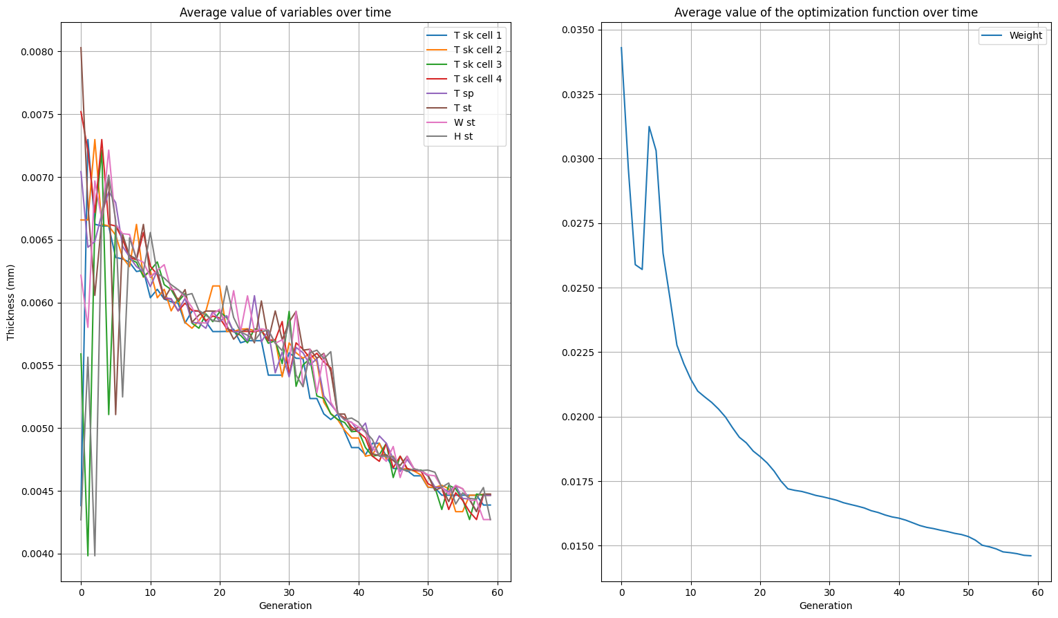
We can also plot the average value of variables over time and optimization function over time, this gives us an idea of how the variables effect the design. Run the code below:
import matplotlib.pyplot as plt

t_sk_cell1_lst = [np.average(pop.get("X")[:][0]) for pop in pop_lst]
t_sk_cell2_lst = [np.average(pop.get("X")[:][1]) for pop in pop_lst]
t_sk_cell3_lst = [np.average(pop.get("X")[:][2]) for pop in pop_lst]
t_sk_cell4_lst = [np.average(pop.get("X")[:][3]) for pop in pop_lst]
t_sp_lst = [np.average(pop.get("X")[:][4]) for pop in pop_lst]
t_st_lst = [np.average(pop.get("X")[:][5]) for pop in pop_lst]
w_st_lst = [np.average(pop.get("X")[:][6]) for pop in pop_lst]
h_st__lst = [np.average(pop.get("X")[:][7]) for pop in pop_lst]

f_lst = [np.average(pop.get("F")) for pop in pop_lst]

fig, (ax1, ax2) = plt.subplots(1, 2)
fig.set_size_inches(18.5, 10.5)

ax1.plot(t_sk_cell1_lst, label="T sk cell 1")
ax1.plot(t_sk_cell2_lst, label="T sk cell 2")
ax1.plot(t_sk_cell3_lst, label="T sk cell 3")
ax1.plot(t_sk_cell4_lst, label="T sk cell 4")
ax1.plot(t_sp_lst, label="T sp")
ax1.plot(t_st_lst, label="T st")
ax1.plot(w_st_lst, label="W st")
ax1.plot(h_st__lst, label="H st")

ax2.plot(f_lst, label="Weight")

ax1.set_title("Average value of variables over time")
ax2.set_title("Average value of the optimization function over time")


ax1.set_xlabel("Generation")
ax2.set_xlabel("Generation")
ax1.set_ylabel("Thickness (mm)")
ax1.legend()
ax2.legend()
ax1.grid()
ax2.grid()

plt.show()
As you can see, it gets quite messy with all variables in there. One could also argue the information gets lost when taking the average and only plotting the optimum solution would give a better idea. It is left up to the reader to implement this.
Changing the amount of stringers#
In the previous optimization we only optimized for the various thicknesses, however a better solution would be possible when different configuration of stringers are used, or even a different layout of ribs.
TUDuam also provides a method for optimizing for different stringer configuration. This is the outer optimization loop as has been shown earlier in this notebook in figure 2. The API documentation for this functionality can be found here. SectionOpt.full_section_opt interally also used the optimization which we experimented with previously. However, it calls this function for every stringer configuration, hence it is signficantly more computationally expensive.
Additionally, stringers often run along multiple sections and hence we’re not completely free in the amount of stringer in each section.
The method does come with a multiprocess flag which does allow it to see major performance boosts on more powerful platforms. So feel free to give it a try on your local machine. The setup is very similar to GA_optimize.
Unlike for the stringer configuration, this repository does not implememt an optimization of the spanwise rib distribution.
Example: Optimizing the wing of a Cessna 172R#
Let us do an example of how we would design the structure of a complete wing. To keep it computationally bounded we are assuming a 3 cell wingbox with a fixed stringer distribution of 10 stringers per cell. Furthermore, here is some important data on the Cessna 172
Characteristic |
Value |
|---|---|
Wingspan |
11 m |
Aspect ratio |
7.32 |
Surface Area |
16.2 \(m^2\) |
Gross weight |
1110 kg |
To come up with the correct loading per bay we make some oversimplified assumptions to make our life easier for this notebook.
Assumptions#
Constant spanwise drag distribution of 230 N/m
Therefore a linear
Mydistribution (see below)A linear lift distribution which is maximum at the root of the wing.
Hence, a cubic
MxdistributionIgnoring the weight of the wing (conservative)
The functions below will be used to get the correct internal forces for each rib section, as can be inferred from average_fun we assume a constant force over each section. This constant force is taken to be the average value over the entire section.
from scipy.integrate import quad
import matplotlib.pyplot as plt
import numpy as np

def average_fun(fun,
                x_start: float,
                x_end: float
                ):
    """
    Calculate the average value of a function `func` over the interval [a, b].

    Parameters:
    func (function): A function that takes a float and returns a float.
    a (float): Lower bound of the interval.
    b (float): Upper bound of the interval.

    Returns:
    float: The average value of the function over [a, b].
    """
    val, _ = quad(fun, x_start, x_end)
    return val / (x_end - x_start)

def shear_y(span):
  return 5444 - quad(lambda x: 1979 - 1979/5.5*x,  0, span)[0]

def moment_y(span):
  return -9980 + quad(shear_y, 0, span)[0]

def shear_x(span):
  return -1265 + 230*span

def moment_x(span):
  return 3478.75 + quad(shear_x, 0, span)[0]

# print(average_fun(moment_x, 5, 5.5))
# print(moment_y(3))

# x = np.linspace(0,5.5,1000)
# y = np.vectorize(moment_x)(x)
# plt.plot(x,y)
# plt.show()
Creating the section#
We must now create the section to iterate over. See the code below whwere we create the rib locations. You can change the exponent of the slicer variable to alter the distribution of the rib locations
import numpy as np


span = 5.5
S = 16.2
n_sec = 8
chord = S/span
slicer = np.linspace(0,1, n_sec)**1.6
rib_loc = slicer*span

print(rib_loc)
[0.         0.24445888 0.74106076 1.41775058 2.24647615 3.21039028
 4.29781608 5.5       ]
Iterating over each section#
With the rib locations and loads specified we can iterate over all the sections. Please see the code below.
from tuduam.data_structures import Wingbox, Material
import warnings

warnings.simplefilter("ignore")
res_lst = []

for idx, rib_1 in enumerate(rib_loc, start=1):
  if idx == len(rib_loc):
    break
  else:
    rib_2 = rib_loc[idx]

  attr_dict = {
      "n_cell":3,
      "spar_loc_nondim":[0.3,  0.7],
      "str_cell": [10,10,10]
  }

  wingbox_struct = Wingbox(**attr_dict)

  shear_y_sec = average_fun(shear_y, rib_1, rib_2)
  shear_x_sec = average_fun(shear_x, rib_1, rib_2)
  moment_y_sec = average_fun(moment_y, rib_1, rib_2)
  moment_x_sec = average_fun(moment_x, rib_1, rib_2)

  applied_loc = 0.45
  opt = SectionOpt(coord_path, chord, len_sec, wingbox_struct, mat_struct)

  upper_bnds = 7*[0.012]
  lower_bnds = 3*[0.0001] +  [0.003] + [0.001] + 2*[0.003]
  res =  opt.GA_optimize(shear_y_sec, shear_x_sec, moment_y_sec, moment_x_sec, applied_loc, upper_bnds, lower_bnds, pop=20, n_gen= 60,multiprocess= False, verbose= False)
  res_lst.append(res)

  print(f"\n\n======== Results rib section {idx} rib {round(rib_1,2)} to {round(rib_2,2)} ==========")
  print(f"Skin thickness = {np.round(np.array(res.X[:3])*1000,2)} mm" )
  print(f"Spar thickness = {round(res.X[3]*1000,2)} mm")
  print(f"Stringer thickness = {round(res.X[4]*1000,2)} mm")
  print(f"Stringer  width= {round(res.X[5]*1000,2)} mm")
  print(f"Stringer height = {round(res.X[6]*1000,2)} mm")
======== Results rib section 1 rib 0.0 to 0.24 ==========
Skin thickness = [3.13 2.9  2.54] mm
Spar thickness = 3.37 mm
Stringer thickness = 1.0 mm
Stringer  width= 3.15 mm
Stringer height = 6.08 mm
======== Results rib section 2 rib 0.24 to 0.74 ==========
Skin thickness = [2.62 2.83 2.39] mm
Spar thickness = 3.19 mm
Stringer thickness = 1.0 mm
Stringer  width= 3.22 mm
Stringer height = 9.19 mm
======== Results rib section 3 rib 0.74 to 1.42 ==========
Skin thickness = [3.27 2.54 2.03] mm
Spar thickness = 3.02 mm
Stringer thickness = 2.1 mm
Stringer  width= 7.36 mm
Stringer height = 8.75 mm
======== Results rib section 4 rib 1.42 to 2.25 ==========
Skin thickness = [2.26 2.36 1.75] mm
Spar thickness = 3.0 mm
Stringer thickness = 2.78 mm
Stringer  width= 6.16 mm
Stringer height = 8.46 mm
---------------------------------------------------------------------------
KeyboardInterrupt                         Traceback (most recent call last)
Cell In[9], line 31
     29 upper_bnds = 7*[0.012]
     30 lower_bnds = 3*[0.0001] +  [0.003] + [0.001] + 2*[0.003]
---> 31 res =  opt.GA_optimize(shear_y_sec, shear_x_sec, moment_y_sec, moment_x_sec, applied_loc, upper_bnds, lower_bnds, pop=20, n_gen= 60,multiprocess= False, verbose= False)
     32 res_lst.append(res)
     34 print(f"\n\n======== Results rib section {idx} rib {round(rib_1,2)} to {round(rib_2,2)} ==========")

File /opt/hostedtoolcache/Python/3.11.14/x64/lib/python3.11/site-packages/tuduam-2026.8-py3.11.egg/tuduam/structures/optimization.py:637, in SectionOpt.GA_optimize(self, shear_y, shear_x, moment_y, moment_x, applied_loc, upper_bnds, lower_bnds, n_gen, pop, verbose, seed, multiprocess, cores, save_hist)
    621     problem = ProblemFixedPanel(
    622         shear_y,
    623         shear_x,
   (...)    633         self.path_coord,
    634     )
    636 method = GA(pop_size=pop, eliminate_duplicates=True)
--> 637 resGA = minimize(
    638     problem,
    639     method,
    640     termination=("n_gen", n_gen),
    641     seed=seed,
    642     save_history=save_hist,
    643     verbose=verbose,
    644 )
    645 return resGA

File /opt/hostedtoolcache/Python/3.11.14/x64/lib/python3.11/site-packages/pymoo/optimize.py:67, in minimize(problem, algorithm, termination, copy_algorithm, copy_termination, **kwargs)
     64     algorithm.setup(problem, **kwargs)
     66 # actually execute the algorithm
---> 67 res = algorithm.run()
     69 # store the deep copied algorithm in the result object
     70 res.algorithm = algorithm

File /opt/hostedtoolcache/Python/3.11.14/x64/lib/python3.11/site-packages/pymoo/core/algorithm.py:133, in Algorithm.run(self)
    131 def run(self):
    132     while self.has_next():
--> 133         self.next()
    134     return self.result()

File /opt/hostedtoolcache/Python/3.11.14/x64/lib/python3.11/site-packages/pymoo/core/algorithm.py:153, in Algorithm.next(self)
    151 # call the advance with them after evaluation
    152 if infills is not None:
--> 153     self.evaluator.eval(self.problem, infills, algorithm=self)
    154     self.advance(infills=infills)
    156 # if the algorithm does not follow the infill-advance scheme just call advance
    157 else:

File /opt/hostedtoolcache/Python/3.11.14/x64/lib/python3.11/site-packages/pymoo/core/evaluator.py:69, in Evaluator.eval(self, problem, pop, skip_already_evaluated, evaluate_values_of, count_evals, **kwargs)
     65 # evaluate the solutions (if there are any)
     66 if len(I) > 0:
     67
     68     # do the actual evaluation - call the sub-function to set the corresponding values to the population
---> 69     self._eval(problem, pop[I], evaluate_values_of, **kwargs)
     71 # update the function evaluation counter
     72 if count_evals:

File /opt/hostedtoolcache/Python/3.11.14/x64/lib/python3.11/site-packages/pymoo/core/evaluator.py:90, in Evaluator._eval(self, problem, pop, evaluate_values_of, **kwargs)
     87 X = pop.get("X")
     89 # call the problem to evaluate the solutions
---> 90 out = problem.evaluate(X, return_values_of=evaluate_values_of, return_as_dictionary=True, **kwargs)
     92 # for each of the attributes set it to the problem
     93 for key, val in out.items():

File /opt/hostedtoolcache/Python/3.11.14/x64/lib/python3.11/site-packages/pymoo/core/problem.py:170, in Problem.evaluate(self, X, return_values_of, return_as_dictionary, *args, **kwargs)
    167     only_single_value = not (isinstance(X, list) or isinstance(X, np.ndarray))
    169 # this is where the actual evaluation takes place
--> 170 _out = self.do(X, return_values_of, *args, **kwargs)
    172 out = {}
    173 for k, v in _out.items():
    174
    175     # copy it to a numpy array (it might be one of jax at this point)

File /opt/hostedtoolcache/Python/3.11.14/x64/lib/python3.11/site-packages/pymoo/core/problem.py:210, in Problem.do(self, X, return_values_of, *args, **kwargs)
    208 # do the function evaluation
    209 if self.elementwise:
--> 210     self._evaluate_elementwise(X, out, *args, **kwargs)
    211 else:
    212     self._evaluate_vectorized(X, out, *args, **kwargs)

File /opt/hostedtoolcache/Python/3.11.14/x64/lib/python3.11/site-packages/pymoo/core/problem.py:228, in Problem._evaluate_elementwise(self, X, out, *args, **kwargs)
    225 f = self.elementwise_func(self, args, kwargs)
    227 # execute the runner
--> 228 elems = self.elementwise_runner(f, X)
    230 # for each evaluation call
    231 for elem in elems:
    232
    233     # for each key stored for this evaluation

File /opt/hostedtoolcache/Python/3.11.14/x64/lib/python3.11/site-packages/pymoo/core/problem.py:16, in LoopedElementwiseEvaluation.__call__(self, f, X)
     15 def __call__(self, f, X):
---> 16     return [f(x) for x in X]

File /opt/hostedtoolcache/Python/3.11.14/x64/lib/python3.11/site-packages/pymoo/core/problem.py:16, in <listcomp>(.0)
     15 def __call__(self, f, X):
---> 16     return [f(x) for x in X]

File /opt/hostedtoolcache/Python/3.11.14/x64/lib/python3.11/site-packages/pymoo/core/problem.py:29, in ElementwiseEvaluationFunction.__call__(self, x)
     27 def __call__(self, x):
     28     out = dict()
---> 29     self.problem._evaluate(x, out, *self.args, **self.kwargs)
     30     return out

File /opt/hostedtoolcache/Python/3.11.14/x64/lib/python3.11/site-packages/tuduam-2026.8-py3.11.egg/tuduam/structures/optimization.py:437, in ProblemFixedPanel._evaluate(self, x, out, *args, **kwargs)
    434 w_st = x[n_cell + 2]
    435 h_st = x[n_cell + 3]
--> 437 box_copy.load_new_gauge(t_sk_cell, t_sp, t_st, w_st, h_st)
    439 # Perform stress analysis
    440 box_copy.stress_analysis(
    441     self.shear_y,
    442     self.shear_x,
   (...)    446     self.mat_struct.shear_modulus,
    447 )

File /opt/hostedtoolcache/Python/3.11.14/x64/lib/python3.11/site-packages/tuduam-2026.8-py3.11.egg/tuduam/structures/wingbox.py:685, in IdealWingbox.load_new_gauge(self, t_sk_cell, t_sp, t_st, w_st, h_st)
    682         idx = pnl.get_cell_idx(self.wingbox_struct, self.chord) # Find which cell  panel is in
    683         pnl.t_pnl = t_sk_cell[idx] # Assign new thickness
--> 685 self._compute_boom_areas(self.chord)
    686 self.Ixx = self._set_Ixx()
    687 self.Iyy = self._set_Iyy()

File /opt/hostedtoolcache/Python/3.11.14/x64/lib/python3.11/site-packages/tuduam-2026.8-py3.11.egg/tuduam/structures/wingbox.py:632, in IdealWingbox._compute_boom_areas(self, chord)
    630 boom.A = boom_area
    631 # check if it is not a spar boom, this will get a flange addition in the future maybe
--> 632 if not any(np.isclose(boom.x, spar_loc_abs )):
    633     boom.A += self.area_str
    634 if boom.A < 0:

KeyboardInterrupt:
Viewing the results#
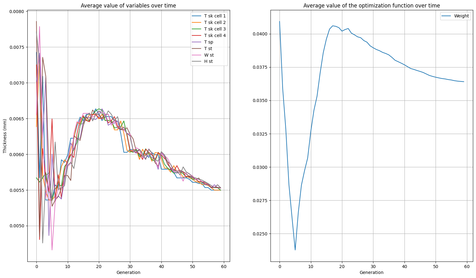
Above you have now seen the final result of each section. The history of each section as we have plotted previously, is also saved in the res_lst variable. The previous code we utilized is wrapped in a function below for easy access such that you can compare the the various sections. Now feel free to change the variables or use the API for your optimizations!
from pymoo.core.result import Result


def plot_history(res: Result):
  pop_lst = [gen.pop for gen in res.history]
  t_sk_cell1_lst = [np.average(pop.get("X")[:][0]) for pop in pop_lst]
  t_sk_cell2_lst = [np.average(pop.get("X")[:][1]) for pop in pop_lst]
  t_sk_cell3_lst = [np.average(pop.get("X")[:][2]) for pop in pop_lst]
  t_sk_cell4_lst = [np.average(pop.get("X")[:][3]) for pop in pop_lst]
  t_sp_lst = [np.average(pop.get("X")[:][4]) for pop in pop_lst]
  t_st_lst = [np.average(pop.get("X")[:][5]) for pop in pop_lst]
  w_st_lst = [np.average(pop.get("X")[:][6]) for pop in pop_lst]
  h_st__lst = [np.average(pop.get("X")[:][7]) for pop in pop_lst]

  f_lst = [np.average(pop.get("F")) for pop in pop_lst]

  fig, (ax1, ax2) = plt.subplots(1, 2)
  fig.set_size_inches(18.5, 10.5)

  ax1.plot(t_sk_cell1_lst, label="T sk cell 1")
  ax1.plot(t_sk_cell2_lst, label="T sk cell 2")
  ax1.plot(t_sk_cell3_lst, label="T sk cell 3")
  ax1.plot(t_sk_cell4_lst, label="T sk cell 4")
  ax1.plot(t_sp_lst, label="T sp")
  ax1.plot(t_st_lst, label="T st")
  ax1.plot(w_st_lst, label="W st")
  ax1.plot(h_st__lst, label="H st")

  ax2.plot(f_lst, label="Weight")

  ax1.set_title("Average value of variables over time")
  ax2.set_title("Average value of the optimization function over time")


  ax1.set_xlabel("Generation")
  ax2.set_xlabel("Generation")
  ax1.set_ylabel("Thickness (mm)")
  ax1.legend()
  ax2.legend()
  ax1.grid()
  ax2.grid()

  plt.show()

plot_history(res_lst[3])