Tutorial: static, buckling, frequency and non-linear analyses of a von Mises truss

This tutorial runs one of the analytic problems of the unit tests of structsolve, the function von_mises_truss of tests/analytic_problems.py, copied below, through the analyses of structsolve: linear static, linear buckling, frequency, and non-linear static with the Newton-Raphson and the arc-length methods.

The shallow von Mises truss of height 1 is loaded through a linear spring of stiffness \(k_s\). The degree of freedom 0 is the apex deflection \(w = c_0\), the degree of freedom 1 the displacement \(c_1\) of the loaded point, and the internal force vector is

\[\begin{split}\boldsymbol{F}_{int} = \begin{Bmatrix} w^3 - 3 w^2 + 2 w + k_s (c_0 - c_1) \\ k_s (c_1 - c_0) \end{Bmatrix}\end{split}\]

with the tangent stiffness matrix \(\boldsymbol{K}_C + \boldsymbol{K}_G\), where \(\boldsymbol{K}_C\) is the linear stiffness matrix and \(\boldsymbol{K}_G\) contains the derivative \(3 w^2 - 6 w\) of the non-linear terms. The truss reaches a limit point at \(w = 1 - 1/\sqrt{3}\), under the limit load \(F_{lim} = 2/(3\sqrt{3})\). The reference load is frac times the limit load.

The model is given to structsolve by the four callables of Analysis, which return the external and the internal force vectors and the two parts of the tangent stiffness matrix:

import numpy as np
import matplotlib.pyplot as plt
from scipy.sparse import csr_matrix

from structsolve import Analysis, freq, lb

frac = 1.5
ks = 10.
F_lim = 2/(3*np.sqrt(3))
w_lim = 1 - 1/np.sqrt(3)
fext = np.array([0., frac*F_lim])
kC = np.array([[2. + ks, -ks], [-ks, ks]])


def calc_fext(inc=1., silent=True):
    return inc*fext


def calc_fint(c, silent=True):
    w = c[0]
    return np.array([w**3 - 3*w**2 + 2*w + ks*(c[0] - c[1]),
                     ks*(c[1] - c[0])])


def calc_kC(c=None, NLgeom=False, silent=True):
    return csr_matrix(kC)


def calc_kG(c=None, NLgeom=False, silent=True):
    w = c[0]
    return csr_matrix(np.array([[3*w**2 - 6*w, 0.], [0., 0.]]))


def analysis(**kwargs):
    an = Analysis(calc_fext=calc_fext, calc_fint=calc_fint, calc_kC=calc_kC,
                  calc_kG=calc_kG)
    for name, value in kwargs.items():
        setattr(an, name, value)
    return an


print('reference load:', fext)

reference load: [0.         0.57735027]

Linear static analysis

Analysis.static(NLgeom=False) solves \(\boldsymbol{K}_{C0} \boldsymbol{c} = \boldsymbol{F}_{ext}\) with the callables calc_kC() and calc_fext():

an = analysis()
increments, cs = an.static(NLgeom=False, silent=True)
c_lin = cs[0]
print('linear solution:', c_lin)

linear solution: [0.28867513 0.34641016]

Linear buckling analysis

The geometric stiffness matrix of the linear solution gives the eigenvalue problem \((\boldsymbol{K}_{C0} + \lambda \boldsymbol{K}_G(\boldsymbol{c}_{lin})) \boldsymbol{u} = \boldsymbol{0}\). With only two degrees of freedom the dense solver is used explicitly, sparse_solver=False, which returns all the load multipliers:

K0 = calc_kC()
KG = calc_kG(c_lin)
eigvals, eigvecs = lb(K0, KG, silent=True, sparse_solver=False)
print('load multipliers:', eigvals)
print('linear buckling estimate of the limit load factor:', eigvals[0])
print('limit load factor:', 1/frac)

load multipliers: [ 1.3494814e+00 -7.2057594e+16]
linear buckling estimate of the limit load factor: 1.3494814008979579
limit load factor: 0.6666666666666666

The linear buckling analysis assumes a linear pre-buckling path, with \(\boldsymbol{K}_G\) proportional to the load. The path of the truss is strongly non-linear before its limit point, and the estimate is here about twice the limit load factor. The non-linear analyses below trace the actual path. The row of the loaded point is null in \(\boldsymbol{K}_G\), and the second load multiplier, of the order of \(10^{16}\), is infinite up to the round-off.

Non-linear static analyses

The Newton-Raphson method controls the load factor, and the arc-length methods of Riks and Crisfield control the arc length, such that the load factor may decrease after the limit point:

results = {}
for method in ['NR', 'arc_length_riks', 'arc_length_crisfield']:
    an = analysis(NL_method=method, initialInc=0.05)
    an.static(NLgeom=True, silent=True)
    results[method] = (np.array(an.increments), np.array(an.cs))
    print('%-21s %3d increments, last load factor %.3f'
          % (method, len(an.increments), an.increments[-1]))

NR                     12 increments, last load factor 1.000
arc_length_riks        18 increments, last load factor 1.000
arc_length_crisfield   14 increments, last load factor 1.000

All the analyses finish at the load factor 1.0. The load-displacement curves of an.increments and an.cs, with the load \(\lambda \, \mathrm{frac} \, F_{lim}\) normalized by the limit load, against the exact equilibrium path \(F = w^3 - 3 w^2 + 2 w\) of the apex:

w = np.linspace(0, 2.3, 200)
fig, ax = plt.subplots(figsize=(6, 4))
ax.plot(w, (w**3 - 3*w**2 + 2*w)/F_lim, 'k-', lw=0.8, label='exact path')
styles = {'NR': 'o--', 'arc_length_riks': 's-', 'arc_length_crisfield': 'x-'}
for method, (inc, cs) in results.items():
    ax.plot(cs[:, 0], inc*frac, styles[method], ms=4, label=method)
ax.axvline(w_lim, color='gray', ls=':', lw=0.8)
ax.set_xlabel('apex deflection $w$')
ax.set_ylabel('load / limit load')
ax.legend()
plt.show()

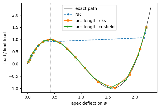
The Newton-Raphson increments follow the path below the limit load and then jump to the inverted configuration, where the load is again larger than the limit load: the analysis converges, but the unstable part of the path is skipped. The arc-length methods pass the limit point, the load factor decreasing and becoming negative during the snap-through, and reach the same final state:

for method, (inc, cs) in results.items():
    print('%-21s largest jump of w: %.3f, final c: %s'
          % (method, np.diff(cs[:, 0]).max(), cs[-1]))

NR                    largest jump of w: 1.889, final c: [2.21463146 2.27236649]
arc_length_riks       largest jump of w: 0.311, final c: [2.21463146 2.27236649]
arc_length_crisfield  largest jump of w: 0.313, final c: [2.21463146 2.27236649]

Frequency analysis along the path

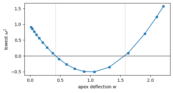
With unit masses at both degrees of freedom, \(\boldsymbol{M} = \boldsymbol{I}\), the frequency analysis of the tangent stiffness matrix \(\boldsymbol{K}_T(\boldsymbol{c}) = \boldsymbol{K}_C + \boldsymbol{K}_G(\boldsymbol{c})\) at each converged state of the Riks analysis gives \(\omega^2 = -\lambda^2\). The lowest \(\omega^2\) vanishes where \(\boldsymbol{K}_T\) is singular, at the limit points \(w = 1 \mp 1/\sqrt{3}\), and is negative between them, where the equilibrium is unstable:

inc, cs = results['arc_length_riks']
M = csr_matrix(np.eye(2))
omega2 = []
for c in cs:
    KT = calc_kC(c, NLgeom=True) + calc_kG(c, NLgeom=True)
    lambda2, _ = freq(KT, M, silent=True, sparse_solver=False,
                      symmetric=True, sort=False)
    omega2.append(-lambda2.max())

fig, ax = plt.subplots(figsize=(6, 3))
ax.plot(cs[:, 0], omega2, 's-', ms=4)
ax.axhline(0, color='k', lw=0.8)
for wl in (1 - 1/np.sqrt(3), 1 + 1/np.sqrt(3)):
    ax.axvline(wl, color='gray', ls=':', lw=0.8)
ax.set_xlabel('apex deflection $w$')
ax.set_ylabel(r'lowest $\omega^2$')
plt.show()