Tutorials#
Defining the Geometry#
Based on the figure:
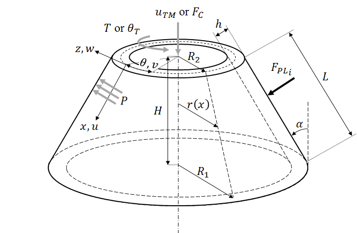
The geometry can be defined using \(H\), \(R_1\) and \(\alpha\), for example, or any other combination (like \(L\), \(H\), \(R_1\)) of the geometric parameters that will allow the complete definition of the cone / cylinder geometry.
Example:
from compmech.conecyl import ConeCyl

cc = ConeCyl()
cc.r1 = 400
cc.r2 = 200
cc.H = 200
Defining the Laminate and Material Properties#
The compmech.composite module is used to calculate the laminate
properties given the stacking sequence, the thicknesses and
the material properties.
The stacking sequence is passed using a container (list or tuple)
with the orientations of each ply, from inwards to outwards:
cc.stack = [0, 0, -45, +45, -30, +30]
The ply thickness is passed using a single value when all the plies have the same thickness or using a container with the thickness of each ply:
cc.plyt = 0.125
or:
cc.plyts = [0.125, 0.125, 0.1, 0.1, 0.101, 0.101]
The material properties are given using a tuple:
where \(E_{11}\) is the elastic modulus along the direction 1 of the ply, \(E_{22}\) the modulus along the direction 2, \(\nu_{12}\) the Poisson’s ratio and \(G_{12}\), \(G_{13}\), \(G_{23}\) the shear modules.
Example:
cc.laminaprop = (123.55e3 , 8.708e3, 0.319, 5.695e3, 5.695e3, 5.695e3)
This will assume the same material properties for each ply. When different
properties must be used the user must supply the laminaprops container.
Example:
prop1 = (123.55e3 , 8.708e3,  0.319, 5.695e3, 5.695e3, 5.695e3)
prop2 = (100.2e3 , 4.2e3,  0.2, 5.1e3, 5.1e3, 5.1e3)
prop3 = (100.2e3 , 4.2e3,  0.2, 5.1e3, 5.1e3, 5.1e3)
cc.laminaprops = [prop1, prop1, prop2, prop2, prop3, prop3]
Linear Static Analysis#
The static analysis is executed using the
compmech.conecyl.ConeCyl.static() method. The following example will
give an overview of the main steps needed for a linear static analysis.
Defining the geometry:
>>> cc.laminaprop = (123.55e3 , 8.708e3,  0.319, 5.695e3, 5.695e3, 5.695e3)
>>> cc.stack = [0, 0, 19, -19, 37, -37, 45, -45, 51, -51]
>>> cc.r2 = 250.
>>> cc.H = 510.
>>> cc.plyt = 0.125
>>> cc.alphadeg = 30.
Defining the model and boundary conditions:
>>> cc.model = 'fsdt_donnell_bc1'
>>> cc.bc = 'cc1'
Defining if the analysis is displacement or load controlled by changing
the boolean parameters pd (prescribed displacement):
prescribed displacement for compression:
cc.pdCprescribed displacement for torsion:
cc.pdTprescribed load asymmetry
cc.pdLA
Applying the axial compression, pressure, torsion and the single-perturbation loads:
>>> cc.Fc = 10000.
>>> cc.T = 100000.
>>> cc.P = -0.01
>>> cc.add_SPL(10.)
>>> cc.add_SPL(4.)
Defining the number of terms in the approximation functions:
>>> cc.m1 = 80
>>> cc.m2 = 40
>>> cc.n2 = 40
Running the analysis:
>>> cc.static()
The results are stored in the cs list, and for a linear static analysis
only one entry exists. Plotting the results:
>>> cc.plot(cc.cs[0], vec='w')
Static Analysis#
where NLgeom is a flag telling whether or not a geometric non-linear
analysis is to be performed.
The solution is stored in the cs attribute, which consists of a list
of 1-D np.ndarray objects. For a linear analysis this list will contain
only one entry while for a non-linear analysis it will contain one entry
for each iteration needed up to the convergence or up to the termination
criterion. To access the last result:
solution = cc.cs[-1]
The displacement field can be plotted, for example:
cc.plot(solution, vec='w', filename='my_output.png')
Non-Linear Analysis#
Using NLgeom=True in a static analysis will run a geometrically
non-linear analysis. Many attributes of the ConeCyl object
are used to control the non-linear analysis (see
ConeCyl.static()).
The converged increments used along the non-linear analysis are stored
in the increments attribute and the corresponding solutions
stored in the cs attribute (a list of 1-D np.ndarray objects).